ESCAPING FROM PREDATORS An Integrative View of Escape Decisions (2015)
Part II Escape and refuge use: theory and findings for major taxonomic groups
IIa Escape theory
2 Theory: models of escape behavior and refuge use
William E. Cooper, Jr.
2.1 Introduction
Despite its crucial role in surviving attacks by predators, escape behavior has received far less theoretical attention from animal behaviorists than other topics, such as foraging and social behavior. Nevertheless, our understanding of escape decisions by prey in certain contexts has been advanced greatly by considering the fitness costs and benefits of escape. Because these costs and benefits of fleeing and hiding have not been measured in fitness units, the models do not permit precise quantitative predictions. They do allow predictions at the ordinal level about effects of greater and lesser levels of factors that affect predation risk and factors that make fleeing costly. Several economic models of escape behavior now routinely provide qualitatively accurate predictions about aspects of fleeing and refuge use. Here, I review these models, develop a model for a scenario not previously treated theoretically, and develop a rubric in which models are placed according to the relative movements of predator and prey. I also discuss alternative approaches to modeling escape decisions and models of behaviors during predator-prey encounters that occur before fleeing.
2.2 First economic models of escape and time spent hiding in refuge
2.2.1 Escape
Much theoretically based empirical research on escape has focused on flight initiation distance (FID), the distance between a prey and an approaching predator when the prey begins to flee (Lima & Dill 1990; Lima 1998; Stankowich & Blumstein 2005). Several other terms are synonyms of FID in some publications, most notably approach distance, flush distance, and flight distance (Chapter 1). Flight initiation distance is the least ambiguous of these terms and is now the most prevalent. The term “flight distance” should be avoided in future research because it is sometimes used to mean flight initiation distance, but in other cases denotes distance fled by the prey. Although escape initiation distance might be preferable to flight initiation distance because some readers might think that flight refers to flying, flight initiation distance is the best of established terms and will be used here.
Economic modeling of escape behavior began with a graphical model by Ydenberg and Dill (1986) that remains useful over 25 years later. Ydenberg and Dill (1986) assumed that prey often do not flee immediately upon detecting (and becoming aware of) an approaching predator, but monitor the predator’s approach until fleeing becomes advantageous. As the distance between predator and prey decreases, the cost of not fleeing increases because the risk of predation increases. Many factors affect the degree of risk at a particular distance. These include the predator’s speed and directness of approach, body size, the prey’s detectability, and body armor (Stankowich & Blumstein 2005; Cooper 2010a). The cost of fleeing is primarily a consequence of losing opportunities to feed, engage in social activities such as courtship, mating, and territorial defense, and to perform other activities that increase fitness. Although usually small, energetic costs of fleeing and risk of injury as a consequence of fleeing are other costs of fleeing. As the predator-prey distance decreases, the opportunity cost of fleeing decreases. This is because less must be foregone by fleeing because the prey has had more time during the predator’s approach to feed, drink, or engage in social activities.
Ydenberg and Dill (1986) proposed that prey begin to flee when cost of not fleeing and cost of fleeing are equal. In their graphical model, flight should occur at the intersection of the falling cost of fleeing and rising risk curves (Figure 2.1). As long as the cost of fleeing is greater than the cost of not fleeing, the prey remains where it is. When the cost associated with predation risk and cost of fleeing are equal, the prey begins to flee because in the next instant cost of not fleeing becomes greater than the cost of fleeing and thereafter the cost of not fleeing grows increasingly larger than the cost of fleeing.
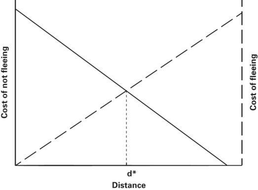
Figure 2.1
Ydenberg and Dill’s (1986) graphical model of flight initiation distance (FID) when a predator approaches an immobile prey that monitors its approach. The horizontal axis is the distance between predator and prey. The vertical axes are the cost of not fleeing, which is primarily expected loss of fitness due to predation risk, and the cost of fleeing, which is incurred when fleeing leads to loss of opportunities to enhance fitness at the prey’s current location. The predicted FID, d*, occurs at the distance where the cost of not fleeing and cost of fleeing curves intersect.
Modified from Ydenberg and Dill (1986)
If the costs were known in exact fitness units, it would be possible to predict flight initiation distance exactly. Ydenberg and Dill’s (1986) model and subsequent economic models are useful because they permit us to make ordinal level predictions about which of two risk levels or which of two costs of fleeing is associated with greater FID. Cost of not fleeing is expressed as cost associated with predation risk or, in shorthand, predation risk.
Many factors affect predation risk (sensu the danger of being killed if no antipredatory behavior is used; Lank & Ydenberg 2003) at a given distance between predator and prey. If two identical predators approach at different speeds, the risk to the prey at any particular distance is greater during the faster approach. If the cost of fleeing is the same in both cases, the cost of not fleeing and cost of fleeing curves intersect farther from the prey when the cost of not fleeing curve is higher (i.e., FID is longer when cost of not fleeing is greater, Figure 2.2b).
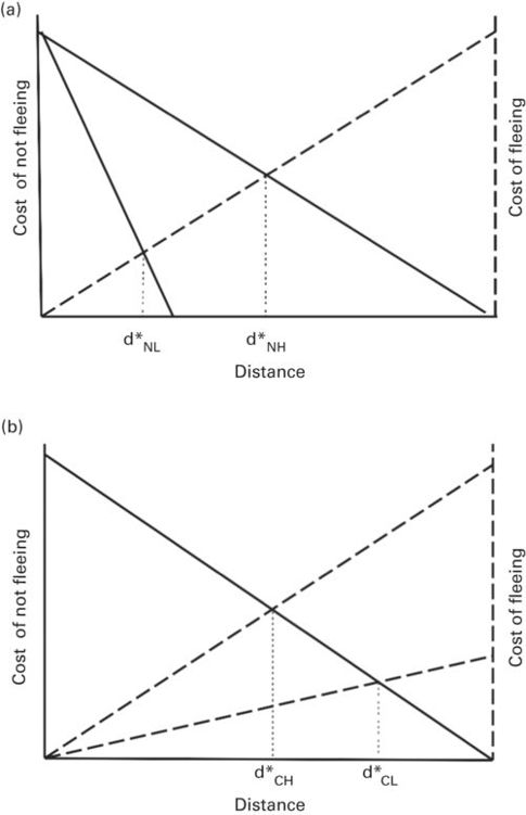
Figure 2.2
The predicted FID, d*, is (A) longer for the higher of two cost of not fleeing curves when there is a single cost of fleeing curve and (B) longer for the lower of two cost of fleeing curves when there is a single cost of not fleeing curve. Terms are d*H for high cost and d*L for low cost.
Modified from Ydenberg and Dill (1986)
If a prey has a feeding opportunity (or other opportunity to enhance fitness), its cost of fleeing is greater at all non-zero distances than that of a prey without a feeding opportunity (Figure 2.2a). Consequently, if the two prey have the same cost of not fleeing curve, the predator is closer to the prey at the intersection of the cost of not fleeing and cost of fleeing curves for the prey having the higher cost of fleeing curve (i.e., FID is shorter when cost of fleeing is greater).
The Ydenberg and Dill (1986) model has been modified by Blumstein (2003) to include three zones (Figure 2.3a). At the shortest predator-prey distances, prey flee as soon as they detect a predator. The shortest zone of predator-prey distance, zone I, extends from distance d = 0 to dmin, the shortest distance at which prey assess risk rather than fleeing immediately upon detecting the predator. In a range of longer distances, zone II, prey make economic decisions based on costs of fleeing and not fleeing as described by Ydenberg and Dill (1986). Zone II extends from dmin to dmax, the maximum distance at which cost-benefit considerations affect escape behavior. (Equivalently, dmax is the maximum distance at which prey assess risk either because they cannot detect the predator or the predator isn’t relevant/poses no risk at longer distances.) Zone III includes all distances longer than dmax. Prey in zone III do not flee. Stankowich and Coss (2007) recognize the same three zones (see also Chapter 3).
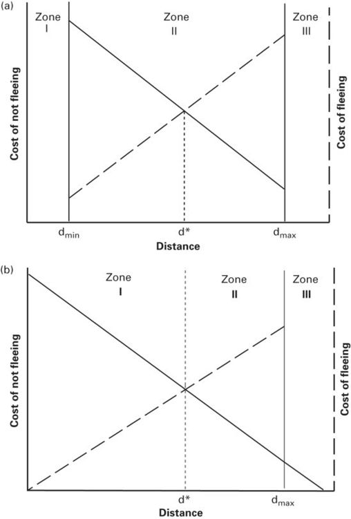
Figure 2.3
Responses of prey to predators differ in three ranges of distance. (A) In Blumstein’s (2003) version, prey flee immediately without assessing risk and cost when they detect predators at close range in zone I. Assessment occurs in zone II, which begins at dmin and continues at all distances in zone II, which ends at dmax. Modified from Blumstein (2003). Prey may or may not detect predators in zone III, but do not monitor them attentively. (B) If prey flee immediately in 0 ≤ d ≤ d*, as predicted by the models of Ydenberg and Dill (1986) and Cooper and Frederick (2007a, 2010), dmin< d* does not exist. Therefore, zone I extends from 0 ≤ d ≤ d*, zone II from d* < d ≤ dmaxand zone III is where d > dmax.
Reasons for non-responsiveness by prey in zone III include failure to detect the predator, inattentiveness to activities at long distance, and the perception that predator-prey distance is too great for the predator to pose an immediate threat (Blumstein, 2003). Stankowich and Coss (2007) added that risk is not assessed in zone III. This is clearly so when the predator is not detected, but is trivial because there has been no predator-prey encounter from the prey’s point of view. On the other hand, prey might appear to be inattentive because perceived risk is too low to justify incurring monitoring costs. An interesting possibility is that prey in zone III that assess risk as being very low nevertheless monitor the activities of predators there, but appear to be inattentive because they monitor predators at intervals rather than continuously, reducing monitoring costs. More empirical work is required to understand the proximate processes occurring in zone III.
Prey are always expected to flee immediately if a predator is detected closer than the economically predicted FID. Therefore the regression of predator-prey distance when the predator is detected on FID should have a slope of 1 on predator-prey distance in the range 0 to d*, the economically predicted FID. A slope that did not differ significantly from 1.0 was observed in the teiid lizard Aspidoscelis exsanguis for approaches starting between 0 and 1.5 m (Cooper 2008). The intercept, too, did not differ significantly from 0 (Cooper 2008). As zone I has been conceived, assessment occurs in the interval between dmin and d*. However, if escape occurs immediately when at d < d*, dmin= d*. In that case zone I is 0 to d*.
If flight begins immediately for d ≤ d*, the zones are modified (Figure 2.3b). Zone 1, the zone of immediate flight, includes distance 0 to d*. In zone II, the zone of monitoring and assessment, d* < d ≤ dmax. In zone III, the non-response zone, the predator is even farther from the prey at d > dmax. Non-response to an approaching threat may indicate either (1) an inability to detect a predator beyond dmax, (2) detection with true lack of any consequent alteration of behavior, or (3) less intense monitoring than occurs in zone II.
Stankowich and Coss (2007) proposed that for prey capable of detecting predators at long distances, higher values of dmax characterize more reactive prey. Such prey would begin cost-benefit assessments at longer predator-prey distances than less reactive prey. Among prey having similar reactivity, scanning rate affects the predator-prey distance at which prey become aware of approaching predators. In Columbian black-tailed deer (Odocoileus hemionus columbianus), 38.5% of individuals had detected investigators before they began to approach, whereas 61.5% became aware some time after approach began (Stankowich & Coss 2007). Because awareness is inferred by an alert posture and orientation to the approacher, this finding is consistent with differences in either reactivity or scanning rate.
The qualitative predictions of Ydenberg and Dill’s (1986) model and the optimal escape model described below have been spectacularly confirmed for diverse prey and factors affecting predation risk and cost of fleeing (Stankowich & Blumstein 2005; Cooper 2010). The models are very useful for predicting decisions about when to begin fleeing by immobile prey that are able to monitor an approaching predator’s behavior and distance. Other models are needed for situations in which prey are moving and both prey and predator are still.
2.2.2 Time spent hiding in refuge
The basic escape model was adapted by Martín and López (1999) from Ydenberg and Dill’s (1986) escape model to predict the time spent by a prey before emerging from a refuge after having been chased into one (Figure 2.4). In the model distance between predator and prey is replaced on the horizontal axis by time spent in refuge and the variable measured is latency to emerge, also called emergence time or hiding time. Hiding time is preferable to emergence time, which also refers to other phenomena, especially times of hatching or metamorphosis.
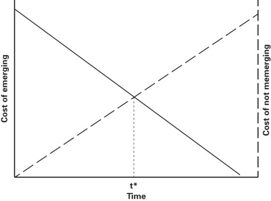
Figure 2.4
The latency to emerge from refuge after fleeing from an approaching predator (hiding time) is predicted to be t*, which occurs at the intersection of the cost of emerging and cost of not emerging curves.
Modified from Martín and López (1999)
The vertical axes of this model are cost of emerging (risk) and cost of not emerging (Figure 2.4). Cost of emerging decreases as time spent in refuge increases because the predator is increasingly likely to have left the area as latency to emerge increases. Cost of not emerging increases as time spent in refuge increases because prey lose opportunities to conduct various activities and, in ectotherms, because body temperature falls during stays in cool refuges, requiring basking or other thermoregulatory behavior upon emergence and decreasing running speed and therefore escape ability (Martín & López 1999; Polo et al. 2005; Cooper & Wilson 2008). A prey is predicted to emerge when the risk of emerging equals the cost of not emerging.
Many of the same predation risk factors and opportunity costs that affect flight initiation distance also affect hiding time. The hiding time model has been particularly successful in increasing our understanding of the effects of thermal costs of refuge use (Martín & López 1999; Polo et al. 2005; Cooper & Wilson 2008). Some empirical studies have shown that risk associated with entering a refuge associated with presence of a predator inside it affects decisions to enter the refuge (Amo et al. 2004).
The hiding time model can be generalized to include effects of the costs of emerging or not emerging due to presence of predators and opportunities outside the refuge, and costs of remaining in or leaving the refuge due to predation risk and opportunities in the refuge (Figure 2.5). In the expanded model, the cost of emerging includes predation risk present in the original model and an additional cost of losing benefits that might be obtained by staying in the refuge. The cost of remaining in the refuge includes both the loss of opportunity available outside the refuge and the risk inside the refuge, primarily due to presence of another predator.
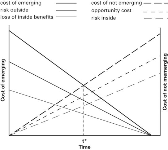
Figure 2.5
If a predator is present outside the refuge and a different predator is inside the refuge, the cost of emerging and cost of not emerging curves each are given by the sum of two costs. The total cost of emerging is the sum of cost due to predation risk outside and loss of benefits that might have been obtained inside the refuge. The total cost of not emerging is the sum of the cost due to risk of predation inside and cost of losing opportunities outside the refuge. The predicted hiding time, t*, occurs at the intersection of the total cost of emerging and total cost of not emerging curves.
The risk of emerging and loss of benefits in the refuge upon emerging decrease as hiding time increases. The opportunity cost and predation risk associated with remaining in the refuge increase as hiding time increases (Figure 2.5). The total cost of emerging is the sum of the cost of emerging due to outside risk and the loss of inside benefits. Similarly, total cost of remaining in the refuge is the cost of lost opportunities outside and predation risk inside the refuge. The predicted hiding time occurs when the total cost of remaining inside equals the total cost of emerging (i.e., at the intersection of the two total cost curves, Figure 2.5). All costs are in expected fitness units. It is apparent that the original hiding time model (Martín & López 1999) is a special case of the model in Figure 2.5 when there are no risks and no benefits to be gained inside the refuge.
2.2.3 Assumptions and restrictions
In both the escape and hiding time models, the cost functions are sometimes shown as linear and sometimes as curvilinear. The precise relationships between predator-prey distance and time spent in refuge and the costs of fleeing or emerging and of not fleeing or emerging are unknown, but the predictions hold for a wide range of functions. As predator-prey distance increases, cost of not fleeing is assumed to decrease and cost of fleeing to increase. However, because cost of fleeing is largely opportunity cost, the cost of fleeing curve may be horizontal or nearly so if opportunity is absent or meager.
Cooper and Vitt (2002) examined these assumptions for the Ydenberg and Dill (1986) model. Their findings are described here for escape, but similar considerations apply to emergence from refuge. Two or more cost of not fleeing curves are assumed to have identical values when predator-prey distance is zero. The cost of fleeing when predator-prey distance is zero is assumed to be zero. Exceptions may occur. If the risk factor is lethality of the predator, the expected loss of fitness is greater for more lethal predators or more vulnerable prey when the predator contacts the prey (Cooper & Frederick 2010). Cost of fleeing at distance zero may be greater than zero for prey that have some chance of surviving contact with a predator, and the cost may differ among predators that impose different opportunity costs, such as differing times spent in refuge.
Imagine that two predation risk curves intersect with each other and intersect at different points with a cost of fleeing curve and that investigators are unaware that the risk curves intersect. Predictions about relative FIDs for the two risk curves based on their magnitudes closer to d = 0 than their intersection would be erroneous because the lower risk curve in this interval intersects the cost of fleeing curve at a longer distance (unless there are multiple intersections between risk curves). For predictions to hold, the cost of fleeing and not fleeing must be monotonic or precisely known. If a non-monotonic cost of not fleeing curve intersects more than once with a risk curve or a non-monotonic risk curve intersects more than once with a cost of fleeing curve, multiple predicted flight initiation distances exist, each for some distance interval.
The graphical models of Ydenberg and Dill (1986) and Martín and López (1999) apply to a wide range of functions relating predator-prey distance or time in refuge to cost curves (Cooper & Vitt 2002). These models have had great heuristic value and have been very successful in empirical tests. Their main theoretical drawback is the requirement that fleeing or emerging can occur only when the curve for cost of not fleeing intersects the curve for cost of fleeing, or the curves for cost of emerging and cost remaining in refuge intersect. This issue is addressed by optimality models.
2.3 Optimality models of escape and refuge use
Optimality models predict that animals select behavioral options that maximize their fitness. In the present context, this implies that prey decide to initiate escape behavior at the FID for which their fitness at the conclusion of the encounter is greatest or to emerge after the hiding time that maximizes fitness when the encounter has ended. Optimality models have been used extensively in studies of foraging behavior (Stephens & Krebs 1986), but only two optimality models of escape have been published, one for FID (Cooper & Frederick 2007a, 2010), the other for hiding time (Cooper & Frederick 2007b). As discussed below, the Ydenberg and Dill (1986) model is not an optimality model because the predicted FID may be associated with less than optimal fitness.
Optimality models of foraging fell out of favor in the mid-1980s for various reasons, especially the presumed inability of animals to make precisely optimal decisions (Stephens et al. 2007). However, they had enormous heuristic value and led to advances in our understanding of foraging behavior and social behavior. For the most part, optimal escape theory is used to make ordinal level predictions, not quantitative ones such as those made by optimal foraging theory. Nevertheless, at our current level of understanding of escape behavior, optimality models, as well as simple cost-benefit models, remain very useful and have led to substantial improvement in our understanding of escape decisions.
In Cooper and Frederick’s (2007a, 2010) optimality model for FID, the optimal FID is the product of predation risk (based on distance) and a term that includes the prey’s initial fitness, benefits that it may gain during the encounter with the predator, and energetic cost of fleeing. All of these terms except initial fitness vary with predator-prey distance, permitting calculation of fitness associated with each flight initiation distance. The optimal flight initiation distance is the predator-prey distance with the highest expected fitness. If all benefits gained during the encounter are lost when the prey is killed, the sum of initial fitness, benefits, and energetic cost is multiplied by the probability of survival to determine expected fitness. However, if benefits are retained after death, as for successful reproduction, fitness is estimated by adding the benefits and energetic costs to the product of the sum of initial fitness and energetic cost with probability of survival.
The prey begins with initial fitness F0. In both the optimality and Ydenberg and Dill (1986) models of FID, benefits are zero at distance dd at the outset of the encounter. The benefit function B(d) increases as the predator draws nearer (i.e., as d decreases). The maximum benefit that may be obtained during the encounter is B*, which is obtained at d = 0. This is because the prey has additional time during the approach to obtain benefits when it allows the predator to come closer. The benefit function in the model is B(d) = B*[1 - (d/dd)n], where dd is the distance at which the prey detects the predator and beyond which benefits cannot be obtained, n is the exponent setting the rate of change in B with respect to d. The benefit function and other terms in the fitness equation might have various mathematical expressions. The energetic expense of fleeing is E(d) = fdm, where d distance, m is the exponent relating expense to d, and f is a proportionality constant that is the slope if m = 1. The probability of survival is 1-e−cd, where c is the rate constant for exponential decay, if contact with the predator is always lethal. These variables and parameters are summarized in Table 2.1.
Table 2.1 Parameters and variable for the optimal flight initiation distance model.
|
B |
benefits in fitness units obtained by the prey during the encounter |
|
B(d) |
function relating benefits obtained to predator-prey distance d |
|
B* |
maximum possible benefits, which are attained at d = 0 |
|
c |
rate constant for exponential decay in probability of survival as d decreases |
|
d |
predator-prey distance |
|
dd |
distance at which the prey detects the predator and at which benefits may start to accumulate |
|
E(d) |
energetic expenditure required to flee when the predator-prey distance is d |
|
f |
proportionality constant affecting energetic expense |
|
F0 |
the prey’s initial fitness (when the encounter begins) |
|
m |
exponent setting the change in energetic expense in conjunction with d |
|
n |
exponent setting the rate of change in benefits with distance |
When all benefits obtained during the encounter are lost if the prey is killed, the prey’s expected fitness if it starts to flee at distance d is F(d) = [F0 + B(d) - E(d)][1 - e−cd], 0 ≤ d ≤ dd. If the prey obtains reproductive benefits or augments fitness by kin selection that are retained if the prey is killed, the equation becomes F(d) = [B(d)] + [F0 - E(d)][1 - e−cd], 0 ≤ d ≤ dd. In the latter equation initial fitness is lost, but the benefits remain.
The optimal FID occurs at the distance where the derivative F′(d) = 0 (and the second derivative < 0, Figure 2.6). Because no analytical solutions for F′(d) exist, the effects of varying model parameters must be studied by simulation. The model predicts that the optimal FID increases as initial fitness and predation risk increase and decrease as benefits increase. The optimal FID decreases as the constant f and the exponent m in the escape cost term decrease due to increasing energetic cost. Only the model that allows retention of benefits predicts that prey should accept great risk or death if benefits are large enough and increase rapidly when the predator is very close.
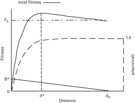
Figure 2.6
In optimal escape theory the prey’s expected fitness increases as benefits that it obtains during the predator’s approach increase. In the absence of predation the total fitness would be the prey’s initial fitness, F0, plus benefits gained at distance d. This total fitness is discounted by the increasing probability of being captured as the predator draws nearer. The distance at which expected fitness is maximized is the optimal flight initiation distance, d*, which decreases as the maximum benefit, B* (obtained by not fleeing), increases and increases as initial fitness increases. The remaining parameter is dd, the predator-prey distance when the prey detects the predator and can start accumulating benefits.
Modified from Cooper and Frederick (2007a)
The optimal FID model has been generalized to account for the degree of predator lethality (Cooper & Frederick 2010) by modifying the term for survival to (1 - L(e−cd), where L is the proportion of fatalities among prey contacted physically by the predator. The optimal FID increases as lethality (L) increases (Figure 2.7). The generalized model can predict FID for factors having complex influences on escape. Consider autotomy, the voluntary shedding of a body part to facilitate escape when overtaken by a predator. Autotomy of the tail by lizards is beneficial because it increases the probability of escape. However, in subsequent encounters with predators, initial fitness is lowered for autotomized individuals because they have decreased reproductive output and growth. Also, lizards that have lost a portion of the tail are less able or unable to use autotomy unless and until the tail has regenerated. Thus predator lethality is greater for autotomized than intact individuals. Decreased ability to obtain benefits and slower running speed by autotomized lizards are predicted to increase FID. Formerly, it was widely believed that FID should increase after autotomy. However, the optimal escape model shows that FID may increase, decrease, or be unaffected by autotomy depending on the balance of effects of autotomy on fitness, lethality, running speed, and ability to obtain benefits.
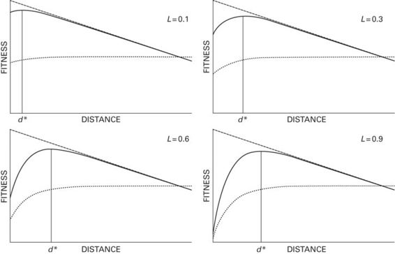
Figure 2.7
For fixed initial fitness, predation risk curve and benefit curve, the optimal FID (d*) increases as the lethality (= L, the proportion of prey that the predator kills upon contact) increases.
Modified from Cooper and Frederick (2010)
The optimal hiding time and FID models are isomorphic. In the optimal refuge use model, time since entering refuge replaces distance as the horizontal axis and in all variables affecting survival and benefits. Optimal hiding time increases as predation risk upon emerging and initial fitness increase and decreases as benefits obtainable upon emerging increase (Cooper & Frederick 2007b).
2.4 Comparison of the graphical and optimality models
Simulations using a range of values for costs, benefits, and initial fitness show that prey can increase their fitness at the end of the encounter to a value greater than their fitness at the outset of the encounter by selecting the optimal FID or hiding time (Cooper & Frederick 2007a,b). This is not possible according to the graphical models discussed above. The best that a prey can do in the graphical models of FID and hiding time is to flee or emerge when the costs of performing the activity equal the costs of not performing it. These graphical models and their mathematical equivalents (Cooper & Frederick 2007a) have been characterized as break-even models to contrast the fitness consequences of the predicted behavioral decisions with those of optimality models, which allow more profitable decisions.
The graphical models do not explicitly consider the prey’s initial fitness, which is an important omission because FID and hiding time are predicted to increase as initial fitness increases according to the asset protection principle (Clark 1993). However, initial fitness could be considered a predation risk factor because more is at risk when initial fitness is greater. Using that approach, graphical models predict longer FID for greater initial fitness, as does optimal escape theory. Qualitative predictions about effects of initial fitness are identical for the break-even and optimality models. Moreover, qualitative predictions of the two types of models are identical for all factors affecting predation risk and cost of fleeing or cost of not emerging.
The two types of models are equally useful for predicting FID and hiding time in almost all circumstances. The only exception occurs when prey can perform activities during the approach or upon emerging from a refuge that allow them to increase their fitness after the encounter to a value greater than its initial level. In some extreme cases this occurs even if the prey dies because it does not flee or because it emerges too soon. For example, a prey might enhance its lifetime fitness by obtaining fertilizations during an approach even at the cost of not fleeing and being eaten. This accounts for prey, such as male black widow spiders (Latrodectus spp.) and male preying mantises (Mantis spp.), that, rather than fleeing, approach their predators to trade their lives for fertilizations.
Cooper and Frederic (2007a) suggested that such cases cannot be accommodated by the Ydenberg and Dill (1986) model because fitness cannot be increased if prey flee when the two cost curves intersect. Consider a graphical model similar to the Ydenberg and Dill model except that cost curves do not intersect. Such cases could be represented by a cost of fleeing curve on which cost of fleeing is greater than the cost of not fleeing at all distances or vice versa (Figure 2.8). Suppose that there is no cost of fleeing or that the cost of fleeing is always less than the cost of not fleeing (Figure 2.8a). Such cases may not exist in zone II. Any intersection would fall in zone III, but would not affect risk assessment. This situation, which may occur when a lethal, efficient predator approaches and no large benefits can be obtained during the encounter. Immediate fleeing is required upon detecting a predator in zone II despite the absence of intersection of the cost curves. This prediction is similar to that of the original zone model (Blumstein 2003) when prey detect predators in zone II closer than the intersection where cost of not fleeing exceeds cost of fleeing. Alternatively, it is similar to the prediction of modified zone model presented above when prey detect predators closer than the optimal FID. The possibility that zone II is longer for more efficient predators has not been studied. The lack of intersection in Figure 2.8b can be interpreted as predicting zero flight initiation distance because cost of fleeing is greater than cost of not fleeing at all distances, which might occur when prey can obtain large reproductive benefits and/or the predator has low lethality or its approach implies low risk.
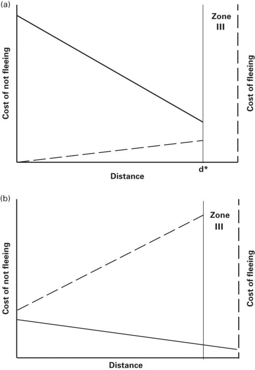
Figure 2.8
Ydenberg and Dill (1986) envisioned cost of not fleeing and cost of fleeing curves whose intersection determined d*, the predicted FID. However, if the curves do not intersect (at least in zone II, the assessment zone) the model applies to broader circumstances. (A) If the cost of not fleeing curve is above the cost of fleeing curve everywhere in the assessment zone, prey should flee as soon as a predator is detected at the boundary of zones II and III, dmax = d*. (B) If the cost of fleeing curve is always higher than the cost of not fleeing curve when d ≥ 0, prey should allow the predator to overtake it. This corresponds to the case in optimal escape theory in which the prey gains enough fitness through reproduction during the predator’s approach to justify loss of fitness expected by contact with the predator.
With the addition of predictions about prey behavior in the cases of non-intersection of the cost curves depicted in Figure 2.8, the Ydenberg and Dill (1986) model and its later modifications discussed above become much more flexible. They apply to all of the situations in the optimality models and make the same qualitative predictions. Quantitative predictions of the graphical and optimality models differ, but that currently is inconsequential because we cannot determine the relevant fitness values. Given fitness values, the relative merits of the models would become an empirical matter. Until the relevant fitness components can be measured, the two types of models may be used interchangeably. The term break-even model, implying that prey flee when expected loss of fitness due to predation risk equals expected fitness gained during the encounter, applies to the graphical models only if the two curves intersect.
2.5 Flushing early: effects of starting distance and alert distance on flight initiation distance
2.5.1 Starting distance: an unexpected challenge to economic escape theory
Starting distance (SD), the predator-prey distance when the predator begins to approach, has an effect on FID that is highly variable and has been difficult to explain. Blumstein (2003) found that FID increased as SD increased in many birds. Since then, SD has been shown to affect FID in mammals (Stankowich & Coss 2007), a crab (Blumstein 2010), and some lizard species (Cooper 2005, 2008; Cooper et al. 2009; Cooper & Sherbrooke 2013a). Among lizards FID did not vary with SD in several species of ambush foragers that were approached slowly (Cooper 2005; Cooper & Sherbrooke 2013a). However, FID increased markedly as SD increased in active foragers (Cooper 2008; Cooper et al. 2009) and, in one ambushing species, increased slightly at fast, but not slow, approach speeds (Cooper 2005).
The effect of SD on FID was difficult to understand, and its basis was controversial. Previously studied factors that affect escape have obvious effects on cost of remaining, cost of fleeing, or both, but the possible effect of SD was obscure. In economic escape theory, a prey monitors a predator as it approaches and decides to flee based on predation risk and cost of fleeing, neither of which are obviously affected by SD.
Blumstein (2010) proposed a possible economic basis in the flush early hypothesis: prey start to flee shortly after having detected a predator to lower the cost of monitoring the predator during its approach. Prey need not flush immediately upon detecting predators, but sometimes do. A recent model suggests that cryptic prey should flee immediately or not at all (Broom & Ruxton 2005). In contrast, in the flushing early model, FID increases as monitoring costs increase. Flushing early matches the effect of SD on FID for a prey that has detected a predator, but is reducing monitoring cost the cause of this relationship?
Spontaneous movement (i.e., leaving its earlier position before a prey detects a predator) might account for an increase in FID with increase in SD, especially for very long SDs. Spontaneous movement also might occur after detection of the predator, leading to increase in apparent FID as SD increases. Such spontaneous movements might generate artifactual increases in the estimates of FID, causing apparent FID to be longer than the FID based on economic decisions. Differences in spontaneous movement rates might account for the differences in effect of SD between ambushing and actively foraging lizards (Cooper 2008). Such differences probably explain some of the difference in effects between foraging modes, but not all, because rates of spontaneous movement by actively foraging lizards are very unlikely to be high enough to account for large effects at short SDs.
The artifactual portion of the effect of spontaneous movement may be reduced or eliminated in prey species that indicate awareness of a predator by staring at and orienting toward it. The predator-prey distance at which this occurs is the alert distance, AD (Blumstein et al. 2005). Because FID is correlated positively with alert distance (Stankowich & Coss 2007), the relationship between SD and FID cannot be entirely due to spontaneous movement by prey that have not detected predators.
Alert distance has its own limitations. Prey may be aware of predators before adopting alert postures and may monitor them less intently then. This may occur when prey detect predators in zone III (Fig. 2.2). Some prey deter pursuit by signaling that they have detected the predator (e.g., Ruxton et al. 2004; Caro 2005; Cooper 2010b, 2011a,b; Chapter 10) and in some cases the signals are alert postures (Holley 1993). In such cases effects of signaling and alert distance per se may be conflated, and this may reduce the apparent effect of alert distance because FID is shorter for signaling than non-signaling prey (Cooper 2011b).
After becoming alert, a prey monitors the predator approaching prior to fleeing. This interval between alerting and fleeing is assessment time (Stankowich & Coss 2007; Chapter 1). The spatial interval corresponding to assessment time is AD to FID (Chapter 1). Monitoring in these intervals matches the scenario of economic models. Alert distance is preferable to SD because larger artifactual effects due to spontaneous movement and statistical constraints (Dumont et al. 2012) occur for SD.
Dumont et al. (2012) examined the relationship between SD and AD for SD ≥ AD to assess the utility of SD as a proxy for AD when AD is difficult to ascertain. By conducting traditional statistical analyses of data for the marmot Marmota marmota using AD as a covariate, they showed that AD and the previous activity of marmots interactively affected FID. Similar analysis using SD as the covariate revealed no such effect. When the assumption that SD ≥ AD ≥ FID ≥ 0 is incorporated into the null hypothesis, SD and AD were unrelated. Dumont et al. (2012) suggested that there is no biologically meaningful relationship between SD and AD. They concluded that SD may be a misleading substitute for AD, but there is no evidence that this conclusion applies widely. They claim that the effect of SD in the range from SD to AD is entirely artifactual. This agrees with the interpretation that spontaneous movements account for any effects of SD in that distance range. However, when SD is short enough for prey to be aware of the predator before the approach begins, the artifact is absent. At longer SDs, use of SD as a proxy for AD is currently the only option when AD cannot be ascertained. As discussed below, it is a viable alternative.
2.5.2 Model of effects of starting distance on flight initiation distance: monitoring costs and spontaneous movements
To examine effects of spontaneous movement and monitoring costs on the relationship between SD and FID, Chamaillé-Jammes and Blumstein (2012) developed a model that predicts two distances, the predator-prey distance where spontaneous movement occurs and FID based on monitoring cost. Recall that dmin in Blumstein’s (2003) model separates zone I where flight is immediate from zone II where escape decisions are based on costs and benefits. Starting distance might or might not affect economic assessment leading to FID in zone II. To allow both possibilities, Chamaillé-Jammes and Blumstein (2012) assumed that the predator-prey distance where monitoring cost elicits escape is proportional to SD. In the equation d* = dmin + βSD, d* is the distance at which prey flee based on monitoring cost and β is the proportionality constant. When β > 0, only spontaneous movement can affect the relationship between SD and FID.
Spontaneous movement was assumed to have a random Poisson distribution with rate λ(s−1), which can also be expressed in m−1. Prey are allowed to move spontaneously when d* < SD. The probability of spontaneous movement increases exponentially as the distance approached by the predator increases. The predicted distance for spontaneous movement is dspon = αeλd, 0 < d* ≤ d ≤ SD, where dspon is the distance where spontaneous movement occurs and α is a proportionality constant. Thus the distance where spontaneous movement is predicted increases exponentially with distance with exponential rate constant λ.
Predicted FID is the longer of the distances predicted separately from monitoring cost and spontaneous movement. Chamaillé-Jammes and Blumstein (2012) applied the model to data from four avian species. They concluded that analysis using ordinary least squares (OLS) is appropriate only if prey move only in response to a predator’s approach. In that case, the slope of the relationship between FID and SD can be tested against the null hypothesis that β = 0. This is an important case because in many studies prey are aware of predators only when an approach begins in zone II. During my extensive field work with lizards, I have the impression that spontaneous movements of many prey are suppressed while monitoring, presumably to reduce the likelihood of being detected and attacked due to their own motion. Suppression of movement during approach is supported by the observation that lizards approached tangentially often flee immediately after passing out of a predator’s field of view (Cooper 1997). In such cases, which include most studies of lizards, OLS analyses are justified.
When the spontaneous (natural) leaving rate λ > 0 and FID is variable at each SD, quantile regression can be used because it permits heterogeneous variances due to differing effects of β and λ across SDs. In OLS procedures, the mean FID is estimated for each value of predator-prey distance. In quantile regression, the value of FID is instead estimated for various quantiles, such as the 10 or 20% of individuals with the lowest or highest values of FID at each SD. This requires a large data set.
For four species of birds with sufficient data using the lowest quantiles (e.g., 5 or 10% of FIDs for a particular predator-prey distance) provided the lowest and best estimates of β. This slope should be 1.0 at distances shorter than dmin, but such distances are excluded from analysis. As λ increases, the slope approaches 1.0. By restricting analysis to the lowest quantiles, many individuals that move spontaneously are excluded, giving a better estimate of the slope of d* on SD based on responses to predators. In two of the four bird species for which FID increased as SD increased using all data, FID was unrelated to SD in quantile regression. When spontaneous movement is frequent and sufficient data are available, quantile regression appears to have great promise (Chapter 17).
2.5.3 Starting distance, alert distance, and economic escape
2.5.3.1 Effects of monitoring predators on escape decisions
Cooper and Blumstein (2014) examined ways in which monitoring might affect FID and proposed novel effects of AD on FID in the context of economic escape theory. Monitoring occurs as part of the scenario in economic escape theory (Ydenberg & Dill 1986; Cooper & Frederick 2007a, 2010), but had not been thought to affect predation risk or cost of fleeing. However, the flush early hypothesis requires that increased monitoring cost associated with longer SD (or AD) causes longer FID (Blumstein, 2010; Chamaillé-Jammes & Blumstein 2012). This can occur only in a limited range of predator-prey distance. If a prey detects an approaching predator in the range 0 ≤ d ≤ d*, economic escape models predict that it should flee immediately. No opportunity exists for dynamic adjustment of FID based on AD at these short distances; AD and related effects of monitoring the predator can affect FID only in zone II where d* < d max.
The effect of monitoring on spontaneous movement can influence the degree to which spontaneous movement affects FID. If movement by the prey increases the likelihood that the predator will attack, spontaneous movements may be suppressed during monitoring. In that case, spontaneous movements occur and the natural rate of leaving, λ, is applicable only for long starting distances in zone III where d > dmax. Spontaneous movement in zone III does not affect estimates of FID in zone II where prey make economic escape decisions. Spontaneous movement occurs in the entire interval between the SD and FID in the model of Chamaillé-Jammes and Blumstein (2012). When this is so, spontaneous movement inflates estimates of FID and methods of removing its effect on FID would be valuable.
Monitoring might affect escape decisions in the cost-benefit escape models via costs of not fleeing and costs of fleeing. The cost of not fleeing is primarily a consequence of predation risk, and increases as the predator comes closer; cost of fleeing is primarily opportunity cost, and increases as FID increases because the prey has less time to complete beneficial activities. Effects of monitoring may be complex, affecting costs of fleeing, not fleeing or both, but have not been studied empirically. Cooper and Blumstein (2014) identified several ways related to SD that monitoring might influence FID. Any combination of the newly identified effects might contribute to flushing early.
2.5.3.1.1 Cost of not fleeing
The physiological cost of monitoring is the energy expended to monitor the predator, presumably via neurological and sensory processes, that is over and above the energy that would be expended in the absence of monitoring. The physiological cost is greater when FID is shorter because the predator has been monitored for a longer time and over a longer distance. Although potentially measurable, it is presumably very small. The total cost of not fleeing is obtained by adding physiological cost to cost due to predation risk (Figure 2.9). Because physiological cost is very small, it can be omitted in empirical studies unless there is reason to believe that it differs among experimental treatments.
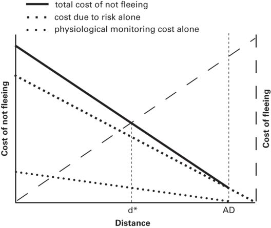
Figure 2.9
Upon detecting an approaching predator at the alert distance, AD, the prey begins to monitor it. The physiological cost of monitoring increases as the duration and distance of approach increase. The sum of this physiological cost of monitoring and the cost due to predation risk is the total cost of not fleeing. The predicted FID, d*, occurs at the intersection of the total cost of not fleeing and cost of fleeing curves. The effect of physiological cost of monitoring is to increase d*.
From Cooper and Blumstein (2014)
The other effect is a dynamic increase in assessed risk as the duration and length of the predator’s approach increase, leading to assessment of greater risk than that attributable to predator-prey distance alone. This effect would lead to increase in FID as AD increases. Prey adjust assessed risk rapidly and dynamically to changes in the behavior of approaching predators (Cooper 2005). As the duration of approach increases, the probability that the predator has detected or will soon detect the prey and will attack increases. Effective risk assessments must account for increased duration/distance approached, which would lead to increase in FID as AD increases.
Alert distance, which affects distance or duration approached, is very likely an important predation risk factor. Alert distance sets limits on the maximum FID and duration of approach during risk assessment. The length of approach and, therefore, assessed risk at any given predator-prey distance increase as AD increases. If duration of monitoring does not affect assessed risk, risk is on the same cost of not fleeing curve for all ADs (Figure 2.10).
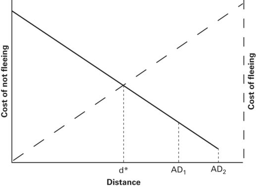
Figure 2.10
The predicted FID, d*, does not vary with alert distance, AD, if the ADs lie on the same cost of not fleeing curve. This would occur if ongoing monitoring does not affect perception of risk dynamically. By projecting the dotted lines vertically from AD1 and AD2 to the cost of fleeing line, it becomes apparent that AD does not affect cost of fleeing when there is a single cost of fleeing curve. This could occur if there is no cumulative cost of monitoring in addition to that incorporated in the cost of fleeing curve.
From Cooper and Blumstein (2014)
A curve representing the case in which assessed risk increases with increase in duration of monitoring lies above the curve for no monitoring cost when 0 < d < AD (Figure 2.11a). Both curves have identical values at AD where assessment begins and at d = 0, where the cost of not fleeing is the expected loss of fitness upon contact with the predator. If the lower curve is linear, the higher risk curve is concave downward (Figure 2.11a). The predicted FIDs are d*N when duration of approach does not influence assessed risk and d*R when it does. The intersection of the cost of not fleeing and cost of fleeing curves occurs at a longer predator-prey distance when assessed risk increases as duration of approach increases than when duration of approach does not affect assessed risk, i.e., d*R> d*N. If assessed risk increases as duration of approach increases and AD differs, the curve for the longer AD, AD2, is above the curve for the shorter AD1 at all d > 0 (Figure 2.11b). In conclusion, when AD affects assessed risk, FID increases as AD increases.
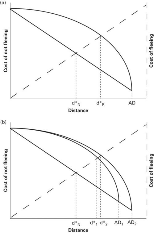
Figure 2.11
In both panels, let a line show the cost of not fleeing when the duration/distance that the predator approaches does not alter the prey’s assessed risk. (A) The upper curve portrays an increase in assessed risk to its maximum at d = 0. For the upper curve, the assessed risk is greater than that in the cost of not fleeing line because the prey assess increasing predation risk as the duration/length of approach increases. The predicted FID, for a prey that that assesses increasing risk as the duration/distance approached increases, d*R, is longer than the predicted FID if alert distance, AD, does not affect assessed risk, d*N. (B) If assessed risk increases as AD increases, assessed risk is greater and the predicted FID is longer for the longer of two ADs.
From Cooper and Blumstein (2014)
2.5.3.1.2 Cost of fleeing
Alert distance might be related to opportunity cost of fleeing in several ways, especially if monitoring entails complete or partial reduction of fitness-enhancing activities. In certain conditions, monitoring does not affect ability to obtain other benefits. For example, basking lizards that have body temperatures too low for efficient locomotion may not feed or engage in social activities. In such cases, FID will not be affected by a monitoring cost associated with a cost of fleeing. This case can be represented by a single cost of fleeing curve with two ADs (Figure 2.10). Because opportunity cost increases as d increases, it is greater at the longer AD. However, the predicted FID is the same for both ADs because they lie on the same cost of fleeing curve (Figure 2.10). This relationship holds for prey that do not flush early because of the monitoring cost of fleeing.
While monitoring predators, prey may not be able to devote sufficient attention to efficiently detect their own cryptic prey (Dukas & Kamil 2000). Suppose that prey have an attentional cost of monitoring and the cost of fleeing curves for prey that do and do not have impaired ability begin at d = 0 and have identical values at AD (Figure 2.12a). The curve for a prey incurring no monitoring cost of fleeing is the highest of a family of such curves. For any two cost of fleeing curves, the curve will be lower for a prey incurring greater monitoring cost. Consequently, for a fixed alert distance, the predicted FID is longer for the curve with greater monitoring costs (Figure 2.12a). The cost of fleeing curve is lowered progressively as the degree of impairment of ability to obtain benefits while monitoring increases.
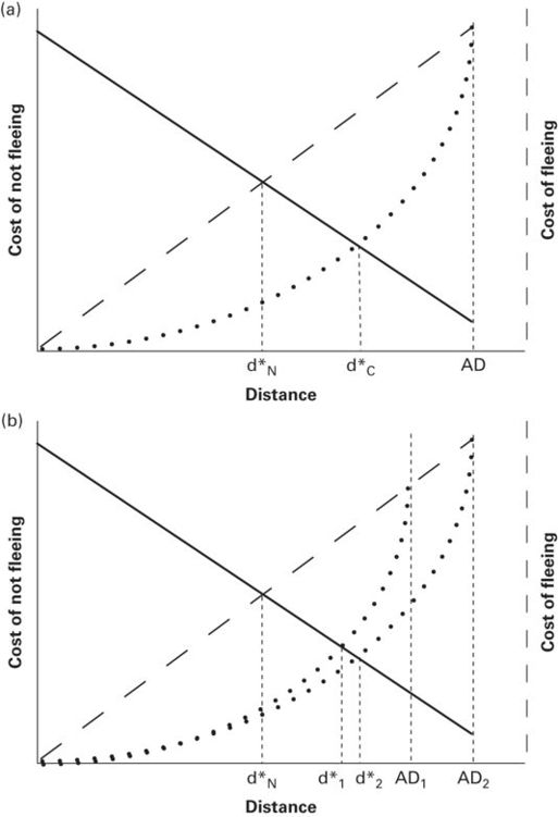
Figure 2.12
(A) Reduced rate of obtaining benefits while monitoring lowers the cost of fleeing and therefore increases FID. This plot shows an upper opportunity cost of fleeing line for a prey that incurs no monitoring cost and a lower curve. In the upper line the opportunity cost is OC0 at d = 0 and OCAD at AD. Monitoring cost is zero for both curves at the origin and at the alert distance (AD), but greater for the lower curve at all distances between them, which lowers opportunity cost of fleeing. In this case the cost of monitoring increases as the predator approaches, but its effect is diminished as benefits remaining to be obtained shrink as predator-prey distance decreases. The predicted FID is shorter for the upper line representing no monitoring cost (d*N) than for the curve in which monitoring impairs ability to obtain benefits (d*C). (B) For two alert distances lying along the line for which monitoring costs do not affect cost of fleeing, let monitoring cost increase at the same rate as duration of approach increases. The cost of fleeing discounted for monitoring cost and adjusted for decrease in remaining benefits as the predator approaches is shown as curves through the origin to two alert distances. The curve for the longer alert distance is always lower than that of the shorter alert distance in the interval 0 < d ≤ AD1, the shorter alert distance. Therefore d* is greater for the longer alert distance. Confirmation of this effect of monitoring on cost of fleeing would strongly support the flush early hypothesis.
From Cooper and Blumstein (2014)
Monitoring cost begins at AD when the prey becomes aware of a threat. At this point, the opportunity cost OCAD is equal for any two curves because no cost of monitoring has accumulated. The cumulative monitoring cost can be calculated by integrating the difference in cost of fleeing between a curve for no monitoring cost and a lower curve for prey having reduced ability to obtain benefits while monitoring between AD and FID. Opportunity cost for all curves at d = 0 is OC0 = 0. Because benefits remaining to be obtained by a prey suffering monitoring cost decrease as predator-prey distance decreases, the total cost of fleeing at a given predator-prey distance is reduced as d decreases, whereas the accumulated cost of monitoring continues to increase. The difference between the two cost curves is progressively reduced toward the origin to account for decline in remaining benefits.
In the same scenario, let two cost of fleeing curves for prey that incur monitoring costs start at different ADs and intersect the cost of fleeing curve for a prey that has no attentional monitoring cost at their respective ADs (Figure 2.12b). The curve having the longer alert distance is always lower than the curve for the shorter alert distance if monitoring cost accumulates at the same rate during the predator’s approach. Therefore the predicted FID is longer for the curve with longer AD (Figure 2.12b). Demonstrating the effects of monitoring and alert distance depicted in Figure 2.12 would provide strong support for the flush early hypothesis.
2.5.3.2 Spontaneous movement
Suppression of spontaneous movement during monitoring would eliminate its effect between AD and FID, but at SD > AD, spontaneous movement increases estimated FID. If prey move spontaneously even while monitoring, empirical estimates of FID will be inflated relative to the economically determined value. The extent of inflation is determined by the natural leaving rate, λ. Using an exponential function as in Chamaillé-Jammes and Blumstein (2012), the proportion of individuals that leave spontaneously between SD and d is 1 - e−λ(SD − d), λ ≥ 0. The estimated FID overestimates the economically based d* by an increasing distance as λ increases and the difference between SD and d* increases. Nevertheless, if AD is held constant in a single population, spontaneous movement does not affect ordinal level predictions of FID for cost of not fleeing and cost of fleeing factors. At the longest observed FID, monitoring costs accumulated during approach are the same for prey that flee and do not flee. Therefore d* must be greater for the prey that flee. The same applies in succession at shorter observed FIDs. In comparative studies, though, differences in λ among species might lead to misinterpretation of findings.
For a prey that has not detected an approaching predator in zone II or III, spontaneous movements occur, but no monitoring costs are incurred before the prey is aware of the predator. For prey that detect the predator at AD, spontaneous movement might continue as monitoring cost is incurred before the predator reaches the economically predicted FID. A major advantage of using AD instead of SD is that spontaneous movements while the prey is not assessing risks and costs are excluded.
Several methods might be used to estimate an economically based FID from raw data that include effects of spontaneous movement. The only method employed to date is discussed in Chapter 16. Other possible methods are suggested here. For normally distributed FID, the highest frequency should occur at d*. The highest frequency should also identify d* if the distribution is skewed to the right as long as the rate of spontaneous movement is not so high that few prey remain when the predator reaches d*. For values of λ that do not drastically deplete prey before the predator reaches d*, the modal FID is presumably d*.
Another method of estimating d* excludes all data for long distances. When d < d*, spontaneous movement does not occur because prey flee immediately, yielding a slope of FID on SD of 1.0. The value of d* can be estimated as the maximum distance for which the slope of FID on SD is 1.0. Although using this method avoids adjustment for spontaneous movement, it would be preferable to estimate d* from data that include spontaneous movements.
Two other methods use data for distances > d*. If the natural rate of leaving is known, the expected proportion of individuals that move spontaneously in each distance interval can be calculated using the exponential relationship presented above. This requires field research to determine whether rates of spontaneous movement are constant across distances, and if so, to estimate λ. Given λ, the expected numbers of individuals that left spontaneously is calculated for distance intervals in which prey do not always flee immediately. Data for the numbers of individuals expected to move spontaneously could then be removed random from each distance interval. The mean FID for the remaining data is an estimate of d*.
A different method of estimating d* is to compare expected proportions of individuals that leave by spontaneous movements with the total proportions that leave in each interval. The longest interval in which the observed proportion that left exceeds the expected proportion to the greatest degree contains d*. In intervals shorter than d*, immediate movement occurs for all individuals, but this is irrelevant in 0 ≤ d < d*.
2.5.3.3 Rapid advances in understanding effects of starting distance
In the short time since Blumstein (2003) reported the effect on SD on FID, SD and AD have been studied intensively. The causes, relationship to economic escape theory, and the effects of spontaneous movement have all been examined theoretically and empirically. Research on relationships among SD, AD, and FID has led to rapid progress in our understanding of these phenomena through the combined theoretical and empirical studies of several behavioral ecologists.
We now understand the basic underlying causes for effects of SD and AD on FID theoretically, but much remains to be discovered, especially about the possible effects of monitoring discussed here on cost of fleeing and on assessed predation risk, and their relationships to flushing early. Research is needed to gauge the importance of all of these potential costs, any or all of which may occur in some prey. Rates of spontaneous movement, their variation with predator-prey distance, and the magnitude of their effect on FID are important topics for future empirical research.
2.6 Other approaches to modeling escape decisions and refuge use
2.6.1 Effect of direction of approach by predator on flight decisions for escape to a fixed refuge
Prey often have options to select among multiple refuges, but in some circumstances only a single refuge is available. There might be only one burrow, tree, or crevice close enough for the prey to reach before being overtaken by a predator. In such cases the direction from which a predator approaches has a strong influence on the risk of being killed if the escape attempt begins at a fixed distance. If the prey is on a line connecting an approaching predator and the refuge, and is located between the predator and the refuge, it can flee directly away from the predator to the refuge (Figure 2.13a). If the prey is on the same line, but the refuge lies between it and the predator, the prey must flee toward the predator to reach the refuge.
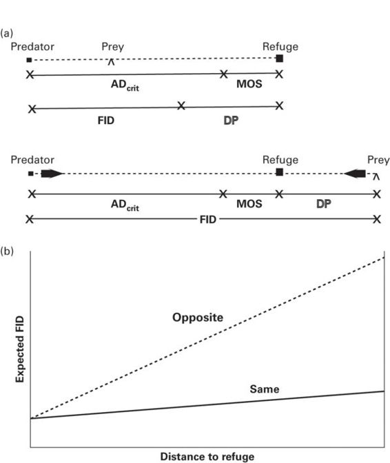
Figure 2.13
Flight initiation distance is shorter when a prey can flee directly away from a predator to a refuge than when it must flee toward a predator t reach refuge. (A)When the prey is between the predator and a refuge and its distance to refuge is DP, its expected FID, FIDexp, is the distance at which predator and prey are expected to reach the refuge simultaneously, ADcrit, plus the a margin of safety, MOS. When the refuge is between the predator and prey and DP and ADcrit are the same as in the previous case, FIDexp must be longer to reach the refuge with the same MOS. For a predator on the same side of the refuge as the prey, FIDexp = ADcrit + MOS - DP; for a predator on the opposite side of the refuge, FIDexp = ADcrit + MOS + DP. (B)The slopes of FIDexp on distance to refuge for predators approaching from the same (solid line) and opposite (dashed line) side of the refuge are shown for MOS = 8 and a predator 1.5 times faster than the prey.
From Kramer and Bonenfant (1997)
Kramer and Bonenfant (1997) modeled the effect of the direction of approach in this situation. They assumed that for both directions, there is a critical predator-prey distance, ADcrit, at which a predator approaching at a fixed speed will reach the refuge at the same time as the fleeing prey. ADcrit stands for critical approach distance, where approach distance is a synonym of FID, and is not to be confused with alert distance. Kramer and Bonenfant (1997) also assumed that prey flee before the predator reaches ADcrit to allow the prey a margin of safety in arrival at the refuge before the predator. In the model, the margin of safety (MOS) is a fixed distance that, when added to ADcrit, gives the predicted FID.
If the prey is between the predator and the refuge, the predicted FID, d*, is ADcrit + MOS - DP, where DP is the distance between the prey and its refuge (Figure 2.13a). If the predator is on the far side of the refuge, the prey must flee toward the predator, requiring a longer FID for equal ADcrit and MOS. The expected FID in this case is d* = ADcrit + MOS + DP (Figure 2.13a). Values of d* vary with distance to refuge, the ratio of predator to prey velocity, and whether the prey is on the same or opposite side of the refuge (Figure 2.13a). Let AV be the velocity of the attacker and PV be the velocity of the prey. Then ADcrit = DP(AV/PV). The slope of the line in Figure 2.13bwhen the predator and prey are on the same side of the refuge (Figure 2.13b) is (AV/PV) − 1, whereas the slope when both the prey and predator are on opposite sides of the refuge is (AV/PV) + 1. These values permit the prediction that these slopes differ by 2.0 slope units. In the only test of this prediction to date, the difference was 1.78 for woodchucks (Marmota monax), which did not differ significantly from 2.0 (Kramer & Bonenfant 1997).
This model complements the cost-benefit model of escape by being mechanistic. It applies only to the risk factors distance to refuge, relative velocities of the predator and prey, and the time/distance until the predator overtakes the prey. Nonetheless, the model makes the same general predictions as economic models (i.e., FID is longer when risk is greater in all three cases). No explicit MOS appears in current economic models, but one must exist for prey to escape contact with predators. Kramer and Bonenfant (1997) did not consider effects of cost of fleeing, but cost of fleeing can be considered to be nearly constant in the absence of social interaction and unusual opportunities by hungry prey to eat scarce food.
The model is remarkable for making predictions solely from readily measured variables, in contrast to economic models that make predictions based on fitness components that are extremely difficult to determine and in practice are not known above an ordinal scale. Further testing is required to determine whether an MOS is constant for a given predator/prey velocity ratio and for approaches from the same and opposite sides. Further testing is also required to determine whether the prediction of the difference of 2.0 slope units applies to other species. Other possibilities, not yet explicitly treated by this or other models, are that prey escape velocities differ when approaching or fleeing away from a predator, and that escape velocities are dynamically adjusted to changes in predator speed.
2.6.2 Game-theoretical model of escape decisions by cryptic prey
When a cryptic prey is approached by a predator, general economic models of FID treat crypsis as a predation risk factor that affects the cost of not fleeing. The more effective the crypsis, the shorter is the predicted FID. Broom and Ruxton (2005) developed a game-theoretical model that applies specifically to the effect of crypsis on FID. Here, the model’s rationale will be discussed; its many equations and parameters can be consulted in the original article.
In the model the prey is aware of the predator before the predator detects the prey, but as the predator draws nearer, its probability of detecting the prey increases. The likelihood of being captured for the prey increases as the predator-prey distance where the predator detects the prey decreases. This scenario differs slightly from that of the Ydenberg and Dill (1986) and optimal escape (Cooper & Frederick 2007a, 2010) models. In those models the effect of decreasing predator-prey distance includes both the increase in probability of being detected and of being caught if attacked, and also allows the predator to have detected the prey before the prey has detected it. However, for a very cryptic prey that has been immobile, it is likely that the prey will detect the predator first.
If the prey flees before it has been detected, it may escape without being detected or its movement may draw the predator’s attention, eliciting an attack. If the prey does not flee when it first detects the predator, but relies on crypsis to avoid being detected and attacked, the risk of being detected is lower than if it flees, but the risk of being captured if detected is greater when the predator is closer upon detecting the prey.
The game-theoretical model includes trajectories and speeds not explicitly stated in the other models and allows consideration of the effect of the prey’s behavior on the predator’s attack strategy. Broom and Ruxton (2005) considered cases in which a predator has passed the prey and can either still see the prey or not and can approach before attacking. Only the case in which the predator is approaching on a straight line and must attack as soon as it detects the prey is describe here.
The game matrix (Table 2.2) includes three possibilities and their payoffs. If no chase occurs, the prey’s payoff is 1 and the predator’s payoff is 0. If fleeing is elicited by attack, the payoffs depend on the predator-prey distance when attack begins, d, the cost of fleeing, c, and the probability of capture when the predator initiates the attack from distance d, f(d), when the predator is at point v on its trajectory. The prey’s payoff is the product of (1 - c) and (1 - f[d(v)]. The predator’s payoff is f[d(v)]. If the prey begins to flee before it is attacked, it gains an advantage in distance covered, Δ, due to the delay in reactive attack by the predator. Therefore when escape is initiated before the predator attacks, the payoffs are (1 - c)(1 - f[d(v) + Δ] for the prey and f[d(v) + Δ] for the predator. The situation in the crypsis model in which delayed escape occurs only when the predator attacks raises questions about how the prey might distinguish continued approach from attack. Prey rapidly adjust FID to changes in speed and directness of approach by predators (Cooper 1997, 1998, 2006), providing possible cues to permit the option of attack-initiated chases for d > 0.
Table 2.2 Payoff matrix of Broom and Ruxton’s (2005) model of escape by a cryptic prey. In the matrix c is the cost of surviving by outrunning the predator, which differs from the opportunity cost of fleeing in economic escape models. The probability that the predator captures if the predator initiates the attack from distance d when at point v on its trajectory is f[d(v)]. The advantage in distance gained by the prey by initiating escape before the predator attacks is Δ.
|
Situation |
Prey’s payoff |
Predator’s payoff |
|
No chase |
||
|
Attack-initiated chase |
(1 - c)(1 - f[d(v)]) |
f([d(v)] |
|
Fleeing-initiated chase |
(1 - c)(1 - f[d(v) + Δ] |
f[d(v) + Δ] |
The major conclusion of the model is that a cryptic prey should either flee immediately when it detects the approaching predator (that is still unaware of the prey) or postpone fleeing until the predator attacks. The prey should flee immediately when the predator has a low search rate (allowing escape with low probability of being detected), cost of escaping by outrunning the predator is low, probability of escaping if the prey initiates escape is greater than if it flees only in response to being detected and attacked, ability to detect the predator at a distance is low, the predator’s ability to detect the prey is greater (ineffective crypsis), and capture rate when the predator attacks is high. In the opposite conditions, prey should postpone fleeing until attacked.
Are the predictions of Broom and Ruxton’s (2005) model consistent with those of general economic escape models? In those models prey should flee immediately whenever the predator is detected closer than the economically predicted FID. If a predator is highly efficient at capturing the prey if it attacks and is unlikely to detect a prey fleeing due to low searching rate, fleeing immediately can be predicted. In the general models, lower cost of fleeing predicts longer FID, but the cost of fleeing is primarily opportunity cost, which is not considered in Broom and Ruxton’s (2005) model. Nevertheless, if c in their model is considered to represent the sum of energetic cost of fleeing, cost of possible injury not inflicted by the predator while fleeing, and opportunity cost, the model is economic. In the general economic models, limited ability to detect the predator increases the likelihood that the predator will not be detected before it reaches the economically predicted FID, and high ability of the predator to detect the prey corresponds to a low degree of crypsis, which predicts longer FID due to greater risk of being detected and attacked.
In the model for cryptic prey, delaying escape attempts until attacked by the predator is favored by low capture efficiency by the predator, high probability of detecting and attacking the prey if it flees, high cost of fleeing if the prey outruns the predator, little or no advantage of initiating escape attempts rather than reacting to attack, strong ability of the prey to detect the predator at long distances, and limited ability of the predator to detect the prey at long distances. All of these factors are associated with shorter predicted FID in the general cost-benefit models through their effects on cost of not fleeing and cost of fleeing.
The predictions of Broom and Ruxton’s (2005) escape model for immediate escape by cryptic prey are consistent with those of Ydenberg and Dill’s (1986) and Cooper and Frederick’s (2007a, 2010) cost-benefit models. The game-theoretical model includes a subset of the predation risk factors in those models. However, predictions of the model for cryptic prey when flight is triggered by attack differ from those of the more general models. The latter predict that prey monitor the predator until it closes to an economically predicted FID that is typically greater than zero. All of the models allow zero FID if crypsis is perfect. However, in the general models, the predicted FID may occur before or after the predator has detected the prey, depending on risk determined jointly by probability of being detected and attacked if detected, and by the predator’s capture efficiency and lethality upon capture. Empirical studies of highly cryptic frogs and lizards (Cooper et al. 2008; Cooper & Sherbrooke 2010a,b) show that some individuals do not flee until overtaken; FID by horned lizards (Phrynosoma cornutum) increased as predation risk (approach speed and directness of approach) increased when the predator did not change speed or directness (Cooper & Sherbrooke 2010a). These findings support the general models in which FID increases with risk and challenge the crypsis model to identify a means of determining how prey assess when attack begins in a manner consistent with the data.
2.6.3 Game-theoretical approach to hiding time in refuge
When a prey flees into a refuge, it may gain safety, but lose information about the predator’s location. A waiting game ensues in which the predator decides whether to stay in the area or seek other prey and the prey decides when to emerge. Emerging too soon may be disastrous for the prey, and waiting too long may be costly to the predator. Due to large differences in fitness consequences for predator and prey, prey are expected to win the waiting game by staying in refuge until after the predator has left the area (Hugie 2003).
Hugie’s (2003) model establishes the existence of an evolutionarily stable strategy of waiting times for predator and prey, the prey’s waiting time being hiding time. The predator’s distribution of waiting times before leaving should resemble a negative exponential distribution, whereas prey should have more variable hiding times and a positively skewed distribution. The model predicts that predators will only rarely outwait prey. The model does not permit predictions about the economic bases of latency to emerge from refuge, but does provides valuable insight into the process leading to successful refuge use.
2.6.4 Stochastic dynamic modeling of fitness consequences of hiding time in refuge
Stochastic dynamic modeling is a technique used to calculate the fitness of animals over some interval of time in which they have made various behavioral decisions (Mangel & Clark 1993), but this useful method of modeling has been applied to decisions about escape and refuge use only once. Rhoades and Blumstein (2007) conducted an empirical study of hiding time and modeled its consequences over the activity season in yellow-bellied marmots (Marmota flaviventris) that must gain sufficient body mass before entering hibernation in order to survive over winter.
The empirical study showed that marmots hide for longer times when approached slowly than rapidly, presumably because their most dangerous predators that stay longer in the vicinity when marmots enter refuge are stalking predators that search specifically for marmots. Hiding time decreased when food was placed outside the burrow. However, the effects of approach speed and added food interacted, being shortest when extra food was present after less risky approaches.
In the model, the ability of marmots to meet their energetic needs is improved, but predation risk is increased, by shorter hiding times. Daily weight gain by different age/sex groups and their asymptotic weights were used to calculate weight upon entering hibernation and daily energetic needs during the activity season. The probability of being killed was considered to be proportional to the amount of time spent outside refuge in each step (90 minute time interval). A proportionality constant, r representing the predation rate in the population was multiplied by the proportion of time in the open to give the probability of predation P = r(t0/t), where to represent time in the open at each step. In the model runs, r was varied between 10 and 50% for the activity season.
Because marmots do not gain energy while in refuge, the amount acquired during each step (i.e., the gain) is g(x) = [kn(t0/t)2], where k is a proportionality constant that was higher when extra food was present and n is units of need. Benefits for prey that emerge early from refuge are elevated by squaring the proportion of time outside refuge to account for high gain by early emergers and loss of the extra food to other group members by late emergers. The net energetic gain G(x) = g(x) - c, where c is the energetic cost (expenditure) in the step. Nine discrete levels of body condition of marmots ranged from 0 (dead) to 8 (able to hibernate without starving to death). Fitness of a marmot at the final step was represented by a sigmoidal function, T (fit) = s2/(4 + s2), where s is the condition.
The model calculated the optimal hiding decisions for an individual over a given number of time steps. To examine effects of suboptimal hiding times on fitness, (1) predation was randomized to permit predation even on prey making optimal decisions and (2) populations of 100 marmots were simulated that used hiding times that were optimal, 50% of optimal, and 200% of optimal.
The consequence of shortened hiding time was drastic: all individuals were killed by predators. Individuals that hid too long lost condition over time, resulting in high mortality (c. 64 to 92%). Survival by prey making optimal decisions was 100% despite inclusion of randomized predation in the model. Thus the stochastic dynamic model highlights the crucial nature of making optimal decisions about hiding, decisions that balance the effects of predation risk against long-term energetic needs. The model revealed differences among age/sex groups in relative hiding times among combinations of approach speed and provision of extra food (or not). The rankings of hiding time for these combinations varied with body conditions both within and among age/sex groups (Rhoades & Blumstein 2007). The model was highly successful in identifying fitness consequences of suboptimal hiding times and revealed subtle variation among age/sex groups and states of body condition that correspond to testable predictions. Stochastic dynamic modeling shows great promise and could readily be applied to trade-offs between hiding time and reproductive and aggressive behaviors and to assessing fitness consequences of suboptimal escape decisions, especially about FID.
2.7 Behaviors prior to fleeing and flight initiation distance: vigilance, alarm calling, and pursuit-deterrent signaling
Several behaviors that may affect escape decisions are omitted or treated in less detail in this chapter, which is devoted to models of escape behavior and refuge use in which prey base decisions on economic considerations and to closely allied models. Vigilance, alarm calling, and pursuit-deterrent signaling are among these behaviors that occur prior to escape. They are considered here theoretically and discussed more comprehensively in Chapter 10. Vigilance affects escape decisions because less vigilant prey may permit predators to approach closer than more vigilant prey would before fleeing. In such cases, more vigilant individuals begin to escape at the longest predator-prey distance where cost of not fleeing outweighs the cost of fleeing. Less vigilant prey may fail to detect the predator until it is closer than the economically predicted distance where escape should begin.
In terms of escape theory, vigilant prey may detect an approaching predator in zone II, in which case it flees when the predator reaches the economically predicted FID, or in zone I, where immediate escape is predicted. A less vigilant prey may not detect the predator until it penetrates zone I, later than would occur for a more vigilant prey. Therefore FID is shorter for the less vigilant of two prey in zone I. Furthermore, predation risk is greater upon detection of a predator for the less vigilant prey. Not allocating time to vigilance can be catastrophic for a prey if it fails to detect the predator until captured. Even if a less vigilant prey flees when it detects a predator that is already close or that flees upon detecting a fleeing conspecific, the increase in risk compared to that for a more vigilant prey can be substantial (Lima 1994).
Many prey signal that they have detected a predator and are able to escape if attacked, or at least more able to escape than non-signaling prey. Nur and Hasson (1984) considered pursuit deterrence to be a case of the handicap principle (Zahavi 1975), which states that some traits that appear to be deleterious have evolved because they demonstrate that the bearer can overcome the handicap, which therefore indicates its superior fitness. Signaling to a predator might be considered a handicap that increases the likelihood of the signaler being detected and attacked. Nur and Hasson (1984) showed that if a signaler has a higher probability of escaping if attacked than nearby conspecifics, a predator should preferentially attack non-signalers. In Nur and Hasson’s (1984) model and in other models unless stated otherwise, prey are aware that a predator is present and direct the signal to that predator.
Game theory is applicable to pursuit deterrence because the fitness consequences for the prey are affected by the predator’s decision to attack or not and the predator’s success depends on the relative escape ability of prey that signal and do not signal. Vega-Redondo and Hasson (1993) employed a game-theoretical approach to model a predator choosing which prey to attack from a herd. The herd includes individuals that have variable signal strength and non-signalers. The prey vary in ability to escape if attacked, which is honestly indicated by signal strength. The predator’s choice also is affected by the frequencies of prey with high and low escape ability that is correlated signal strength. Given these conditions, an equilibrium favorable to both predator and prey exists, in part because a cheater whose signal indicates greater escape ability than it possesses is likely to be captured if attacked, which occurs at some probability greater than zero. At equilibrium, strong signalers are less likely to be attacked and predators gain attacking weaker signalers. The probability of successful cheating increases as herd size increases and the frequency of high-quality prey decreases, which affects the equilibrium probabilities of signaling and attacking.
Alarm calling by prey that detect predators may evolve by kin selection even if calling increases the chances of being detected and attacked. Signaling may also have a pursuit-deterrent function if the signaler is likely to escape because it is aware of the predator. In a game-theoretical model of alarm calling called the watchful babbler game (Bergstrom & Lachman 2001), the payoff matrix has separate entries when a predator is present and absent and, when a predator is present, separate entries for prey that do and do not signal (Table 2.3). When a predator is absent, uncertain prey may signal with payoff 1 - c, where c is the prey’s cost of signaling. If the prey does not signal, its payoff is one. In both cases the payoff for the predator is 0. If a predator is present and the prey signals, the prey’s payoff is (1 - c)(1 - t), where t is the probability of being captured if the predator attacks. The predator’s payoff in this situation is t - d, where d is the cost to the predator of attacking. If the prey signals, but the predator does not attack, the prey’s payoff is 1 - c and the predator’s is zero. When the prey does not signal and the predator attacks, the payoff is 1 - t for the prey and t - d for the predator. Finally, if the prey does not signal when a predator is present but fails to attack, the prey’s payoff is 1 and the predator’s payoff is 0. The predator’s maximum possible payoff in this model is the same for prey and predator.
Table 2.3 Payoff matrix of the watchful babbler game in which the prey can signal or not in the presence or absence of a predator and the predator can attack or not whether the prey signals or not. The prey’s payoff is 1, its current fitness, if it does not signal and is not attacked. The predator’s payoff is 0 if it does not attack and t - d if it attacks, where t is the probability of capturing the prey that it attacks and d is the cost of attacking. The maximum payoff for the predator is the prey’s fitness and can only be achieved if capture is certain and attack carries no cost.
|
Predator present |
||||||
|
Signal |
No signal |
Predator absent |
||||
|
Chase |
No chase |
Chase |
No chase |
Signal |
No signal |
|
|
Prey |
(1 - c) (1 - t) |
1 - c |
1 - t |
1 - c |
||
|
Predator |
t - d |
t - d |
||||
Modified from Table 1 in Bergstrom and Lachmann (2001)
A key feature of this model is that the prey is uncertain whether a predator is present or not, and is more likely to signal when it assesses the probability of a predator being present to be higher. The model predicts that calls may not only inform conspecifics about the presence of a predator, but also honestly inform the predator that it has been detected and that the signaler is therefore more likely to escape if attacked. The signal does not indicate that signalers have greater physiological escape ability, only that they are aware. In Bergstrom and Lachmann’s (2001) model, the cost of signaling is a consequence of alerting predators other than the one to which the prey is responding to the prey’s presence. The watchful babbler game has a stable equilibrium at which predators are less likely to attack when prey signal. At equilibrium, prey benefit by being less likely to be attacked and killed, whereas predators benefit by not incurring cost of attacking when the probability of capture is too low.
An unpublished game-theoretical model by W. Cooper and W. Frederick examines effects of a predator on prey’s decision to signal and of a solitary prey on the predator’s decision to attack. The model makes four assumptions. First, signal strength does not vary. Second, the probability that a prey that has signaled will be killed if the predator attacks, Ks, is lower than that for a prey that does not signal, Kns. Thus signaling is honest (Kns - Ks > 0). If the term Kns - Ks is zero, signaling is not beneficial to predator or prey. Third, units in the payoff matrix are fitnesses for predator and prey normalized to 1. Fourth, the cost of signaling for the prey, Cs, is very small compared to the benefit of a kill for the predator, B (i.e., Cs << Bk). In effect, the benefit of the kill is unaffected by the signaling cost to the prey.
The game matrix (Table 2.4) excludes the case in which no predator is present that was in the payoff matrix of the watchful babbler game (Table 2.3). The model assumes that the predator has been detected with certainty. The optimal signaling strategy for the prey depends on the probability that the predator will attack, and the optimal attack strategy by the predator depends on the probability that the prey signals. Thus the equilibrium strategies in the pursuit deterrence game are determined by mutual influences of predator and prey. The model is derived in ESM 2.1, which is available at www.cambridge.org/9781107060548.
Table 2.4 Payoff matrix of a game-theoretical model of pursuit deterrence for solitary prey that are certain that a predator is present. The predator attacks with probability p and does not attack with probability 1 - p. The prey signals with probability q and does not signal with probability 1 - q. For each combination of predator and prey actions, the payoff for the predator is shown first, separated by a comma from the payoff for the prey. B - the predator’s benefit from killing the prey, Ca - the predator’ cost of attacking, Cs - the prey’s cost of signaling, Ks - the probability of killing a prey that has signaled if the predator attacks, Kns - the probability of killing a prey that has not signaled if the predator attacks.
|
Prey |
|||
|
Signal (q) |
Not signal (1 - q) |
||
|
Predator |
Attack (p) |
(BKs - Ca, 1 - Ks - Cs) |
(BKns - Ca, 1 - Kns) |
|
Not attack (1 - p) |
(0, 1 - Cs) |
(0, 1) |
|
(Cooper & Frederick, unpublished)
Pursuit-deterrent signaling is relevant to escape decisions if signaling lowers the probability of being attacked and, therefore, predation risk. The models of pursuit deterrence show that honest signals that communicate the prey’s likelihood of escaping when aware of the predator lead to a stable equilibrium of signaling and attack with reduced probability of attack on signalers. The reduced risk associated with signaling predicts that a prey should allow a predator to approach closer before fleeing when the prey signals than when it does not. This prediction was confirmed in the zebra-tailed lizard, Callisaurus draconoides, that lizards that signaled allowed predators to approach closer before they fled than did non-signaling individuals (Cooper 2011b).
2.8 Escape latency
The models considered thus far predict FID by an immobile prey being approached by a predator and hiding time in refuge when a predator was known to be nearby upon refuge entry. Two recent graphical models (Martín et al.2009; Cooper et al. 2012) predict latency to flee by an immobile prey near an immobile predator. The former model is limited to predictions about effects of risk factors on escape latency. The latter model applies to predation risk factors and opportunity costs and is similar to the Ydenberg and Dill model of FID when a predator moves toward an immobile prey.
The escape latency model applies when a prey has moved toward an immobile predator before stopping or a predator has moved toward an immobile prey before stopping. If the prey has not detected the predator while approaching it or while the predator has approached the prey, the standing distance may be shorter than the economically predicted FID when the prey has monitored the predator’s approach. Therefore the escape latency model applies to a wide range of standing distances, the distance between the immobile predator and immobile prey. Because an immobile prey might approach the predator after a period of immobility, the prey’s latency to approach might also be modeled and measured, but is not considered here beyond noting that a prey may assess the immobile predator as posing less risk as time spent immobile increases.
The encounter begins when the prey becomes aware that an immobile predator is nearby. Escape latency is the time between initial awareness and initiation of escape behavior. In the graphical model (Cooper et al. 2012; Figure 2.14) escape latency (time) is the horizontal axis and the cost of fleeing and cost of remaining immobile (not fleeing) are the left and right vertical axes, respectively. Cost of fleeing decreases as escape latency increases because the predator is increasingly likely to detect and attack the prey. Cost of immobility increases as time increases because opportunity cost increases. The predicted escape latency occurs at the intersection of the increasing cost of remaining immobile and the decreasing cost of fleeing curves.
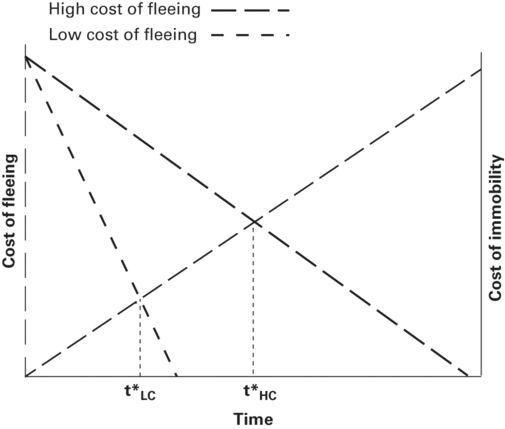
Figure 2.14
When an immobile predator is near an immobile prey, the probability that the predator will detect and attack the prey increases with time. Therefore the cost of fleeing incurred when movement causes the prey to be detected and attacked decreases as time increases. Cost of remaining immobile increases as time increases due to increasing loss of opportunities to enhance fitness that require movement. The predicted latency to flee, t*, occurs at the intersection of the two cost curves. Escape latency model. From Cooper et al. (2012). Predicted latency to flee, t*, is longer for the higher of two cost of fleeing curves. Although not shown, it also is longer for the lower of two cost of immobility curves intersecting a single cost of fleeing curve.
Cost of fleeing decreases as risk increases. For two costs of fleeing (e.g. those for fast versus slow approach speeds by the predator), the latency to escape is predicted to be greater when predation risk is smaller (cost of fleeing is higher).Latency to flee is greater when standing distance is greater because risk is lower at longer standing distance due to longer time required by a predator to detect the prey and lower risk of being captured if attacked. Prey are predicted to move sooner when cost of remaining still is higher, preventing them from obtaining benefits of feeding, social behavior, or other activities that increase fitness. If expected benefits are large enough relative to risk, a prey animal may not flee, but instead approach the predator to obtain the benefit or move toward the source of benefit without approaching the predator. In such cases the variable measured is latency to move or latency to approach the predator, not escape latency.
Only a few tests of predictions of the models of escape latency have been conducted because the models are new; tests are thus far limited to lizards. However, all predictions tested have been verified. Escape latency is affected by standing distance and many of the predation risk factors known to affect FID. It increases as standing distance increases (six species), predator approach speed before stopping decreases (three species), directness of approach by the predator decreases (three species), for the second of two consecutive approaches (two species), and is greater when the predator maintains eye contact with the prey than looks elsewhere (one species) (Martín et al. 2009; Cooper et al. 2012; Cooper & Sherbrooke 2013b). Escape latency decreases when opportunities to enhance fitness are present. It is shorter in the presence than absence of food (two species) or an unfamiliar female that may be courted by males (one species) (Martín et al. 2009; Cooper et al. 2012; Cooper & Sherbrooke 2013b). In all cases in which an effect has been observed in two or more species, two families and both active foraging and ambush foraging modes are represented, hinting that the predictions may apply to prey from diverse taxa having disparate ecological traits. More research is needed on additional taxa.
2.9 New model of nearest approach distance by a prey approaching an immobile predator
In a previously unmodeled scenario, a prey approaches an immobile predator that the prey has detected (Figure 2.15). As in Ydenberg and Dill’s (1986) model of FID, the horizontal axis in the graphical model of nearest approach distance is distance between prey and predator. Left and right vertical axes are the cost of approaching and cost of not approaching, respectively. The cost of approaching due to predation risk increases as the distance from the predator decreases. The cost of not approaching, which is primarily an opportunity cost incurred when some benefit can only be obtained by approaching the predator, increases as distance from the predator increases. This model applies only to prey that have sensory systems and cognitive abilities that allow them to perceive an immobile preditor. The model is not applicable to prey that lack these abilities, such as some teiid lizards that often approach and walk on the feet of people who have remained immobile for some time.
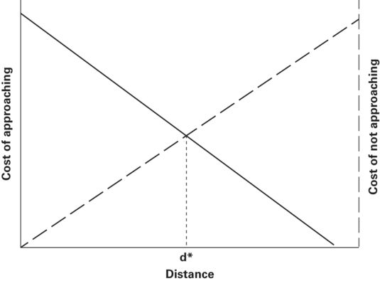
Figure 2.15
A prey approaching an immobile predator must balance the increasing cost of approaching (risk of predation) as it draws nearer against the cost of not approaching, which is primarily an opportunity cost. This model is isomorphic to Ydenberg and Dill’s (1986) model of FID (Figure 1) with cost of approaching substituted for cost of not fleeing and cost of not approaching for cost of fleeing.
The prey is predicted to stop approaching when the costs of approaching and not approaching are equal, which occurs at the intersection of the cost curves (Figure 2.15). This may be accomplished by becoming immobile or moving in a different direction to avoid coming too close. The predictions for two cost of approaching or two cost of not approaching curves are similar to those of Ydenberg and Dill’s (1986) FID model (Figure 2.2) and Cooper et al.’s (2012) latency to flee model (Figure 2.14). The higher of the two cost of approaching curves intersects with a single cost of not approaching curve at a greater distance, indicating that the predicted nearest approach distance is longer when predation risk is greater. The intersection of the higher of two cost of not approaching curves with a single cost of approaching curve is closer to the predator than that of the lower cost of not approaching curve. This comparison shows that the predicted nearest approach distance is shorter for higher cost of not approaching curves.
Mathematical expression of the Ydenberg and Dill (1986) model and related graphical models varies with the nature of cost curves. As a first approximation, linear cost curves can be used (Cooper & Frederick 2007a). The fitness cost of approaching the predator until distance d = 0 is the prey’s initial fitness, F0, multiplied by the predator’s proportional lethality (L), which is LF0. Let the cost of approaching be a negative linear function of predator-prey distance, A(d) = LF0 - ad, where a > 0 is the slope of the fitness cost of approaching the predator on distance from the predator. The derivative is A′(d) = - a and is the marginal cost of approaching, which increases from zero where the cost of approaching line intersects the distance axis to LF0 when d = 0. The cost of not approaching, N(d) is zero at d = 0 and increases linearly as predator-prey distance increases (N(d) = nd, where n > 0 is the slope of the cost of not approaching on predator-prey distance). The marginal cost of not approaching is N′(d) = n.
The prey should continue its approach while the cost of not approaching exceeds the cost of approaching. If the cost of approaching is greater than or equal to the cost of not approaching, the prey should stop approaching. The model predicts that approach continues until A(d) = N(d), which occurs at the predicted nearest approach distance, d*. For linear cost of approaching and not approaching curves, d* = LF0/(n + a).
Greater cost of approaching at a particular distance corresponds to a higher cost of approaching curve and longer nearest approach distance, implying a lower absolute values of the slope a. Suppose that costs are linear and two cost of approaching lines have slopes -a and -a^, and a > a^. The difference in predicted nearest approach distance for the lines that intersect a single cost of not approaching line is d*^ - d* = LF0(a - a^)/[(n + a)(n + a^)]. The difference a^ - a is positive because a^ < a, corresponding to greater nearest approach distance for the cost line having the lower slope, a^.
The greater of two costs of not approaching at a particular predator-prey distance is associated with the slope n^ > n. For two cost of not approaching lines that intersect a single cost of approaching line, the difference in predicted nearest approach distances is d*^ - d* = LF0(n - n^)/[(n + a)(n^ + a), where d* is the predicted nearest approach distance for slope a. The nearest approach distance is shorter for a steeper cost of not approaching line (n^ > n).
In the Ydenberg and Dill (1986) model of escape, the cost of not fleeing could be represented by any function that decreases monotonically or is non-increasing as predator-prey distance increases; similarly any monotonically increasing or non-decreasing function might be considered as a possible cost of fleeing curve (Cooper & Vitt 2002). Non-linear curves for cost of approaching must be described by monotonically decreasing or non-increasing functions of distance and those for cost of not approaching must be described by monotonically increasing or non-decreasing functions of distance.
Here, I describe one non-linear cost of approaching. As a prey approaches a predator, risk may increase slowly at long distances from the predator, but accelerate rapidly near the predator, resulting in a steeper rise in cost of approaching when nearing the predator. In such cases the cost of approaching may be a negative exponential function of distance, A(d) = LF0e−cd, where c is the rate constant for exponential decay. The cost of approaching is the expected fitness if contacted by the predator times the probability of being killed if the prey stops approaching at d. If cost of not approaching is linear and cost of approaching is negative exponential, the predicted nearest approach distance is d* = LF0/n - d*/e−cd = d*ecd*. The solution of this equation is d* = ProductLog (cLF0/n)/c, where the function ProductLog(z) in Mathematica is the principal solution for w in z = wew. As when both cost functions are linear, d* depends on lethality, initial fitness, and the rate constants for decrease in risk and increase in cost of not approaching as distance increases. Provided that risk approaches zero for a negative exponential cost where a linear cost reaches the distance axis, risk is lower for the negative exponential cost than the linear one at all distances except d = 0. Therefore the cost of approaching curve intersects the cost of not approaching line closer to the predator (i.e., nearest approach distance is shorter for the negative exponential than the linear cost of approaching).
An advantage of the model is that it allows many testable predictions to be made for diverse prey. The model permits a wide range of predictions to be made for many of the risk factors that affect decisions to flee or emerge from refuge in other scenarios. Each of the factors affects the degree of risk incurred by approaching the predator. Among these are longer nearest approach distance (1) for direct than indirect approach, (2) for prey that encounter predators infrequently than for prey habituated to the presence of potential predators that do not attack, (3) for the second of two approaches if attacked during the first approach, (4) for longer than shorter distance to refuge, (5) for longer than shorter starting distance, (6) for the more conspicuous prey or prey in less concealing cover, (7) for prey with less effective body armor or other effective defenses, and (8) for slower prey. Predictions are clear for other risk factors such as numbers of predators and prey, predator and prey sizes, direction of the predator’s gaze, etc. Among factors affecting the cost of not approaching, shorter nearest approach distance is predicted for hungry prey in the presence than absence of food, for reproductively active prey in the presence than absence of mating opportunities, for thirsty prey in the presence than absence of water, and for hypoxic prey in a gradient of oxygen concentration that increases as distance from the predator decreases, and for prey that encounter more favorable thermal conditions nearer the predator.
The model’s predictions may be more difficult to test than those of models for the scenarios discussed above. In the other escape scenarios, the prey is immobile, permitting a researcher or a model of a predator to approach the prey in various ways that affect risk or to approach to a desired position and then remain still. Collecting data on nearest approach distance in the field often may require a researcher to move to a location where prey are likely to approach and then remain immobile while waiting to be approached. Because there is no advantage of a researcher being able to move toward prey, predator models may be used more frequently. Tests of the model could be facilitated by studying highly mobile prey that spend a high proportion of the time moving, such as active foragers. If approaches by prey are infrequent, data could be accumulated by using motion-activated video recorders.
2.10 Relative movement of prey and predator: escape variables and models
Economic models of decisions about escape, refuge use, and approaching a predator share the perspective that prey adjust antipredatory behavior to both predation risk and costs of the antipredatory activities. Risk is traded for benefit in all of the models. Each model applies to a particular scenario defined by the movement of both predator and prey, and predicts a behavioral variable appropriate for the relative movements (Table 2.5). The first models described in this chapter were developed to predict FID when a predator approaches an immobile predator (Ydenberg & Dill 1986; Cooper & Frederick 2007a, 2010). More recently models were published that predict escape latency when both predator and prey are immobile (Martín et al. 2009; Cooper et al. 2012). In the preceding section, I presented a model that predicts how closely a moving prey will approach an immobile predator before stopping or changing its direction of movement.
Table 2.5 Models predicting escape decisions for various scenarios of relative movement and location of a prey and a single predator.
|
Movement/location |
||||
|
Prey |
Predator |
Variable |
Model |
Source |
|
still |
moving |
FID |
graphical |
Ydenberg and Dill 1986 |
|
optimality |
Cooper and Frederick 2007a, 2010 |
|||
|
still |
still |
latency to flee |
graphical |
Martin et al. 2009, |
|
Cooper et al. 2012 |
||||
|
PAL |
graphical |
this publication |
||
|
moving |
still |
NAD |
graphical |
this publication |
|
moving |
moving |
not developed |
none |
none |
|
in refuge |
outside |
hiding time |
graphical |
Martín and López 1999 |
|
optimality |
Cooper and Frederick 2007b |
|||
FID: flight initiation distance; MAD: nearest approach distance; PAL: prey approach latency.
The only scenario not yet modeled is escape or approach by prey when both the predator and the prey are moving. This scenario is the most complex of the possibilities shown in Table 2.5. Relative speeds and directions of predator and prey are important when both are moving. If they are moving away from each other, risk decreases, requiring no additional behavioral alteration by the prey. If they are moving closer to each other, maximum risk is influenced by the minimum bypass distance between predator and prey if their trajectories are maintained. If the minimum bypass distance is long enough, prey may not alter their movements. When the minimum bypass distance is shorter, prey might be predicted to stop farther from the predator, as in the model of nearest approach distance, but the nearest approach distance should then be longer than if the predator were immobile. If the prey stops moving, the scenario shifts to that of FID models.
When both predator and prey are moving, prey have options other than stopping (which would shift the encounter to the original scenario of Ydenberg and Dill 1986), such as changing trajectories to avoid coming closer to predators, fleeing in various directions, and entering refuge. A prey might alter its speed rather than its trajectory to increase the minimum bypass distance, or alter both speed and trajectory. Degree of predation risk associated with the predator’s speed relative to that of the prey, lethality, and other factors affecting risk may be predicted to affect the predator-prey distance at which prey change their speed, direction, or both, as well as the magnitude of the changes. The effects of foraging, social, and other opportunities should be to decrease the predator-prey distance when the prey’s behavior is altered and decrease changes in speed and direction of movement. If the predator alters its movements to attack, the focus shifts from decisions by prey prior to being attacked to a later stage of predator-prey encounters, pursuit.
For linear trajectories, the slopes of the lines and the speeds determine whether, when, and where intersection occurs. Nearest approach distance can be calculated using parametric equations of the vector values to determine distances between predator and prey and then determine its minimum value, which occurs when the derivative of distance is zero. However, because predator and prey are free to change their trajectories, a linear model would have very limited applicability. On the other hand, it might be possible to use such a model to predict when a prey should alter its path and/or speed given a linear approach by the predator. We know little of such dynamics prior to pursuit. It would be worthwhile to use video recording to assess the responses of prey approaching a manipulatable model predator that in turn approaches the prey.
2.11 Conclusions
Theory is now available to guide empirical studies of many aspects of escape behavior. Cost-benefit models have been very successful in making predictions about effects of factors that influence cost of fleeing and cost of not fleeing on FID and latency to flee, and about costs of emerging and not emerging from refuge on hiding time. The new model I presented here provides similar predictions about the nearest approach distance for a prey approaching an immobile predator.
Some escape variables have been neglected in escape models, especially the distance fled, escape speed, escape trajectory when the predator does not pursue, and the probability of entering a refuge. Both distance fled and probability of entering refuge are expected to increase as predation risk increases and cost of fleeing decreases. However, the distance to the nearest refuge may affect both decisions. These relationships have not been modeled formally. Nevertheless, predictions for distance fled and refuge entry made using the logic of the economic models of FID have often been verified (Cooper 2009). However, there are exceptions (Cooper 2009). Although some exceptions could be consequences of unrecorded variation in distance to refuge, closer empirical examination of these variables is needed. Theory to guide research on relationships between these variables and costs and benefits would be very useful to inform such research.
Optimality models analogous to that for FID (Cooper & Frederick 2007a, 2010) and hiding time (Cooper & Frederick 2007b) could easily be developed for latency to flee and nearest approach distance. I have not done so here because almost all of their ordinal level predictions are the same as those of the graphical FID model by Ydenberg and Dill (1986). However, the optimality models allow the prey to make better escape decisions, and would be useful in theoretical studies of fitness.
Several other topics relevant to escape have received no theoretical attention. Models predicting the precise effects of alarm calling and other forms of pursuit-deterrent signaling on FID would be useful. Escape trajectories and speeds prior to pursuit have been largely ignored theoretically for terrestrial prey, but theory and empirical findings about trajectories are presented in Chapter 8, with emphasis on aquatic prey. The complex case in which both predator and prey are moving, but pursuit has not begun, will require explicit consideration of speeds and directions of movement by both predator and prey. Models and empirical studies of this scenario would greatly expand our knowledge of escape behavior. Another area in which our theoretical understanding is limited is the pursuit phase of predator-prey encounters, which is discussed in Chapter 8.
References
Amo, L., Lopez, P. & Martin, J.(2004). Multiple predators and conflicting refuge use in the wall lizard, Podarcis muralis. Annales Zoologici Fennici, 41, 671-679.
Bergstrom, C. T. & Lachmann, M. (2001). Alarm calls as costly signals of antipredator vigilance: The watchful babbler game. Animal Behaviour, 61, 535-543.
Blumstein, D. T. (2003). Flight-initiation distance in birds is dependent on intruder starting distance. Journal of Wildlife Management, 67, 852-857.
Blumstein, D. T. (2010). Flush early and avoid the rush: A general rule of antipredator behaviour?Behavioral Ecology and Sociobiology, 21, 440-442.
Blumstein, D. T., Fernández-Juricic, E., Zollner, P. A. & Garity, S. C. (2005). Inter-specific variation in avian responses to human disturbance. Journal of Applied Ecology, 42, 943-953.
Broom, M. & Ruxton, G. D. (2005). You can run or you can hide: Optimal strategies for cryptic prey. Behavioral Ecology, 16, 534-540.
Caro, T. M. (2005). Antipredator Defenses in Birds and Mammals. Chicago: University of Chicago Press.
Chamaillè-Jammes, S. & Blumstein, D. T. (2012). A case for quantile regression behavoral ecology: Getting more out of flight initiation distance data. Behavioral Ecology and Sociobiology, 66, 985-992.
Cooper, W. E., Jr. (1997). Factors affecting risk and cost of escape by the broad-headed skink (Eumeces laticeps): Predator speed, directness of approach, and female presence. Herpetologica, 53, 464-474.
Cooper, W. E., Jr. (1998). Direction of predator turning, a neglected cue to predation risk. Behaviour, 135, 55-64.
Cooper, W. E., Jr. (2005). When and how does starting distance affect flight initiation distance. Canadian Journal of Zoology, 83, 1045-1050.
Cooper, W. E., Jr. (2006). Dynamic risk assessment: prey rapidly adjust flight initiation distance to changes in predator approach speed. Ethology, 112, 858-864.
Cooper, W. E., Jr. (2008). Strong artifactual effect of starting distance on flight initiation distance in the actively foraging lizard Aspidoscelis exsanguis. Herpetologica, 64, 200-206.
Cooper, W. E., Jr. (2010a). Economic escape. In Encyclopedia of Animal Behavior, Vol. 1. London: Academic Press, pp. 588-595.
Cooper, W. E., Jr. (2010b). Pursuit deterrence varies with predation risks affecting escape behaviour in the lizard Callisaurus draconoides. Animal Behaviour, 80, 249-256.
Cooper, W. E., Jr. (2011a). Influence of some potential predation risk factors and interaction between predation risk and cost of fleeing on escape by the lizard Sceloporus virgatus. Ethology, 117, 620-629.
Cooper, W. E., Jr. (2011b). Pursuit deterrence, predations risk, and escape in the lizard Callisaurus draconoides. Behavioral Ecology and Sociobiology, 65, 1833-1841.
Cooper, W. E., Jr. & Blumstein, D. T. (2014). Starting distance, alert distance and flushing early challenge economic escape theory: New proposed effects on costs of fleeing and not fleeing. Behavioral Ecology, 25, 44-52.
Cooper, W. E., Jr. & Frederick, W. G. (2007a). Optimal flight initiation distance. Journal of Theoretical Biology, 244, 59-67.
Cooper, W. E., Jr. & Frederick, W. G. (2007b). Optimal time to emerge from refuge. Biological Journal of the Linnaean Society, 91, 375-382.
Cooper, W. E., Jr. & Frederick, W. G. (2010). Predator lethality, optimal escape behavior, and autotomy. Behavioral Ecology, 21, 91-96.
Cooper, W. E., Jr. & Sherbrooke, W. C. (2010a). Initiation of escape behavior by the Texas horned lizard (Phrynosoma cornutum). Herpetologica, 66, 64-71.
Cooper, W. E., Jr. & Sherbrooke, W. C. (2010b). Plesiomorphic escape decisions in cryptic horned lizards (Phrynosoma) having highly derived antipredatory defenses. Ethology, 116, 920-928.
Cooper, W. E., Jr. & Sherbrooke, W. C. (2013a). Effects of recent movement, starting distance and other risk factors on escape behaviour by two phrynosomatid lizards. Behaviour, 150, 447-469.
Cooper, W. E., Jr. & Sherbrooke, W. C. (2013b). Risk and cost of immobility in the presence of an immobile predator: Effects on latency to flee or approach food or a potential mate. Behavioral Ecology and Sociobiology, 67, 583-592
Cooper, W. E., Jr. & Vitt, L. J. (2002). Optimal escape and emergence theories. Comments on Theoretical Biology, 7, 283-294.
Cooper, W. E., Jr. & Wilson, D. S. (2008). Thermal cost of refuge use affects refuge entry and hiding time by striped plateau lizards Sceloporus virgatus. Herpetologica, 64, 406-412.
Cooper, W. E., Jr., Caldwell, J. P. & Vitt, L. J. (2008). Effective crypsis and its maintenance by immobility in Craugastor frogs. Copeia, 2008, 527-532.
Cooper, W. E., Jr., Wilson, D. S. & Smith, G. R. (2009). Sex, reproductive status, and cost of tail autotomy via decreased running speed. Ethology, 115, 7-13.
Cooper, W. E., Jr., López, P., Martín, J. & Pérez-Mellado, V. (2012). Latency to flee from an immobile predator: Effects of risk and cost of immobility for the prey. Behavioral Ecology, 23, 790-797.
Dukas, R. & Kamil, A. (2000). The cost of limited attention in blue jays. Behavioral Ecology, 11, 502-506.
Dumont, F., Pasquaretta, C., Réale, D., Bogliani, G. & Von Hardenberg, A. (2012). Flight initiation distance and starting distance: Biological effect or mathematical artefact. Ethology, 118, 1051-1062.
Holley, A. J. F. (1993). Do brown hares signal foxes? Ethology, 94, 21-30.
Hugie, D. M. (2003). The waiting game: A “battle of waits” between predator and prey. Behavioral Ecology, 14, 807-817.
Kramer, D. L. & Bonenfant, M. (1997). Direction of predator approach and the decision to flee to a refuge. Animal Behaviour, 54, 289-295.
Lank, D. B. & Ydenberg, R. C. (2003). Death and danger at migratory stopovers: problems with “predation risk”. Journal of Avian Biology, 34, 225-228.
Lima, S. L. (1994). On the personal benefits of vigilance. Animal Behaviour, 48, 734-736.
Lima, S. L. (1998). Stress and decision making under the risk of predation: recent developments from behavioral, reproductive, and ecological perspectives. Advances in the Study of Behavior, 27, 215-290.
Lima, S. L. & Dill, L. M. (1990). Behavioral decisions made under the risk of predation: a review and prospectus. Canadian Journal of Zoology, 68, 619-640.
Mangel, M. & Clark, C. W. (1993). Dynamic Modeling in Behavioral Ecology. Princeton, NJ: Princeton University Press.
Martín, J. & López, P. (1999). When to come out from a refuge: Risk-sensitive and state-dependent decisions in an alpine lizard. Behavioral Ecology, 10, 487-492.
Martín, J., Luque-Larena, J. J. & López, P. (2009). When to run from an ambush predator: Balancing crypsis benefits with costs of fleeing in lizards. Animal Behaviour, 78, 1011-1018.
Nur, N. & Hasson, O. (1984). Phenotypic plasticity and the handicap principle. Journal of Theoretical Biology, 110, 275-297.
Polo, V., López, P. & Martín, J. (2005). Balancing the thermal costs and benefits of refuge use to cope with persistent attacks from predators: A model and an experiment with an alpine lizard. Evolutionary Ecology Research, 7, 23-35.
Rhoades, E. & Blumstein, D. T. (2007). Predicted fitness consequences of threat-sensitive hiding behavior. Behavioral Ecology, 18, 937-943.
Ruxton, G. D., Sherratt, T. N. & Speed, M. (2004). Avoiding Attack: The Evolutionary Ecology of Crypsis, Warning Signals and Mimicry. Oxford: Oxford University Press.
Stankowich, T. & Blumstein, D. T. (2005). Fear in animals: A meta-analysis and review of risk assessment. Proceedings of the Royal Society of London, Series B, Biological Sciences, 272, 2627-2634.
Stankowich, T. & Coss, R. G. (2007). Effects of risk assessment, predator behavior, and habitat on escape behavior in Columbian black-tailed deer. Behavioral Ecology, 18, 358-367.
Stephens, D. W. & Krebs, J. R. (1986). Foraging Theory. Princeton, New Jersey: Princeton University Press.
Stephens, D. W., Brown, J. S. & Ydenberg, R. C. (2007). Foraging. Chicago: University of Chicago Press.
Vega-Redondo, F. & Hasson, O.(1993). A game-theoretic model of predator-prey signaling. Journal of Theoretical Biology, 162, 309-319.
Ydenberg, R. C. & Dill, L. M. (1986). The economics of fleeing from predators. Advances in the Study of Behavior, 16, 229-249.
Zahavi, A. (1975). Mate selection: A selection for a handicap. Journal of Theoretical Biology, 53, 205-214.