The Philosophy of Physics (2016)

7
Quantum Philosophy

Quantum mechanics is our best theory of the material world. It has been applied successfully to three of the four interactions of nature (electromagnetic, strong, and weak), and work continues apace to apply it to gravitation. Scott Aaronson ([1], p. 110) describes quantum mechanics as not so much a physical theory, but as something falling halfway between a physical theory and a piece of pure mathematics. He uses the analogy of an operating system [OS], where the procedure of making a theory quantum mechanical (i.e. quantizing) amounts to ‘porting’ the application (e.g. Maxwell’s classical theory of electromagnetism) to the OS. One might extend his analogy by thinking of quantum mechanics itself as a significant ‘upgrade’ from classical (Newtonian) mechanics, which proved unable to ‘run’ certain programs. All of our quantum theories are achieved through this porting procedure: one starts off with a known classical theory and then performs some specific modifications to it.1

Porting an application into the quantum OS brings along with it a whole bunch of curious features that did not appear on the older OS: indeterminacy, matter waves, contextuality, non-individuality, decoherence, entanglement, and more. These features still account for the vast majority of work done within the philosophy of physics, though recent work done on ‘quantum computation’ has altered their flavour somewhat. Other recent work on quantum theory has tended to focus on specific issues of quantum fields, especially the issue of the extent to which the theory contains particles. These more advanced issues must wait until the next, final chapter. For now we focus on the ‘classic’ philosophical problems of quantum mechanics, and get to grips with its basic features. The four core problems we focus on are: the interpretation of probability and uncertainty; the measurement problem; the problem of nonlocality; and the problem of identity. These overlap and splinter in a great variety of ways, as we will see. Firstly, let us motivate some of the basic oddities of quantum mechanics.

7.1 Why is Quantum Mechanics Weird?

I’m sure that anyone reading this book will have heard all of the sayings about how strange quantum mechanics is. The quotes from famous physicists are legion: ‘if you think you understand quantum mechanics, then you don’t understand quantum mechanics.’ In his popular book on quantum electrodynamics, Richard Feynman puts it like this:

What I am going to tell you about is what we teach our physics students in the third or fourth year of graduate school - and you think I’m going to explain it to you so you can understand it? No, you’re not going to be able to understand it. Why, then, am I going to bother you with all this? Why are you going to sit here all this time, when you won’t be able to understand what I am going to say? It is my task to convince you not to turn away because you don’t understand it. You see, my physics students don’t understand it either. That is because I don’t understand it. Nobody does. ([14], p. 9)

Often, amongst physicists of a certain stripe, thinking about the meaning of quantum mechanics is a violation of some unwritten rule of what physicists are supposed to do. Or worse, it might lead one into philosophy talk! The slogan is: ‘shut up and calculate!’

But quantum mechanics is a physical theory. Experiments demonstrate quite clearly that it applies (even if it is ultimately only an approximation) to the world (the actual world): our world! Surely it ought to be understandable? We ought to be able to say something about how the theory latches (with such impressive empirical success) onto the systems in this world. That is, there ought to be some interpretation of the theoretical formalism that enables us to see how the theory ‘works its magic.’ There is no such thing as magic, so there must be some rational, physical account. And indeed there is, or rather are.

There exist very many ways to ‘make sense’ of quantum mechanics: Copenhagen, modal, relative-state, many-worlds, many-minds, Bayesian, Bohmian, Qbist, spontaneous collapse, etc. However, what one person considers to be a perfectly rational account, another might consider to be outright lunacy. There is an almost religious fervour concerning the holding of a particular stance on quantum mechanics: ‘the church of Everett’ versus ‘the church of Bohm’! Let us make a start on finding out what it is people are disagreeing about - it sure isn’t anything experimentally testable, which is why many physicists dismiss the whole business of interpretation as completely irrelevant. However, whatever position one adopts, it is undeniably true that there are elements of quantum mechanics that are genuinely weird, as we will see - but in many ways, no less weird than time dilating and spacetime warping in the context of the theories of relativity. Perhaps the weirdest is the quantum version of the two slit experiment.

As Feynman maintains in his Lectures on Physics, much of the strangeness of quantum mechanics can be seen in the so-called double slit experiment, which he argues is “impossible, absolutely impossible, to explain in any classical way” ([12], p. 1) - indeed, he believes this contains “the only mystery” in quantum mechanics, and one that cannot be gotten rid of by explaining how it works (ibid.): there is no explanation, only (extraordinarily precise, though still probabilistic) prediction. This experiment reveals the interference (wavelike) properties of quantum particles. It is this interference that’s responsible for most of the other curiosities of quantum mechanics - including the speed gains that quantum computers make over classical ones. A similar experiment was used earlier, in 1802, by Thomas Young to demonstrate the wave nature of light (and thus disconfirm Newton’s corpuscular theory) - see fig. 7.1. Quite simply, as the light travels from the two slits, A and B, to the detection screen it will have sometimes shorter and sometimes longer distances to reach the various parts of the screen. There will be cases where light following a short path from one slit coincides with light following a long path from the other slit, and so the light is likely to be out of phase at such points. One can then have either constructive or destructive interference, which will give rise to lighter bands (when the phases add) and darker bands (when the phases subtract) on the screen, at C, D, E, F.

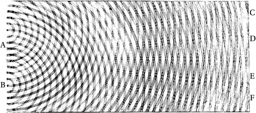
Fig. 7.1 The interference pattern as drawn by Thomas Young for a wave passing through a screen with two slits.

It is one thing for a beam of light to behave in this watery way, but the startling feature of quantum mechanics, known as ‘wave-particle duality,’ is that it also applies to ‘material particles’ too. Inversely, thanks to the duality, particle-like behavior can be found in phenomena more commonly thought to be wavelike (such as light). With modern technology, one can perform these experiments so that only single particles are leaving the source and traveling to the screen, leaving a single click or scintillation where they are detected (see fig. 7.2).

After a small number of detection events the clicks appear to be random. However, on performing many such runs one finds the most startling result: even though the particles are hitting the screen as individual events, over time the old classical wave pattern (as sketched by Young) is built up much as a pointillist painter discretely renders a continuous scene (see fig. 7.3).

Fig. 7.2 The interference pattern after 65 photons have been detected at the screen. This simulation was carried out in Mathematica with a slit separation of 1 cm and a wavelength of light of 560 nm. [Code by S. M. Binder: http://demonstrations.wolfram.com/WaveParticleDualityInTheDoubleSlitExperiment/].

We have used light in this example, but as mentioned above, the same results can be found with electrons and other particles. Indeed, one can even find this kind of behavior for complex structures such as molecules (including organic molecules) consisting of almost 1,000 atoms. The difficulty in ‘supersizing’ the double slit experiment lies in upholding the ‘quantumness’ (quantum coherence) of the objects in the face of decoherence, which destroys the interesting phase (interference) effects through interacting with the environment and its many degrees of freedom.

To add to the oddness of this experiment, when one performs the experiment with just one slit open the strange wave-like pattern vanishes and is replaced by the boring classical buildup one would expect. Yet why does the particle care whether one or two slits are open: surely it goes through one or the other, not both? However, it seems to in some sense go through both - even a single particle - constructively and destructively interfering with itself, and then becoming a point-like particle once again when it reaches some measurement device (such as the detection screen). This apparent measurement-dependence of wave (continuous, linear) versus particle (discrete, non-linear) behavior is part of the quantum measurement problem, and it, rather than superposition itself, standardly supplies the proving-ground of interpretations of quantum mechanics.

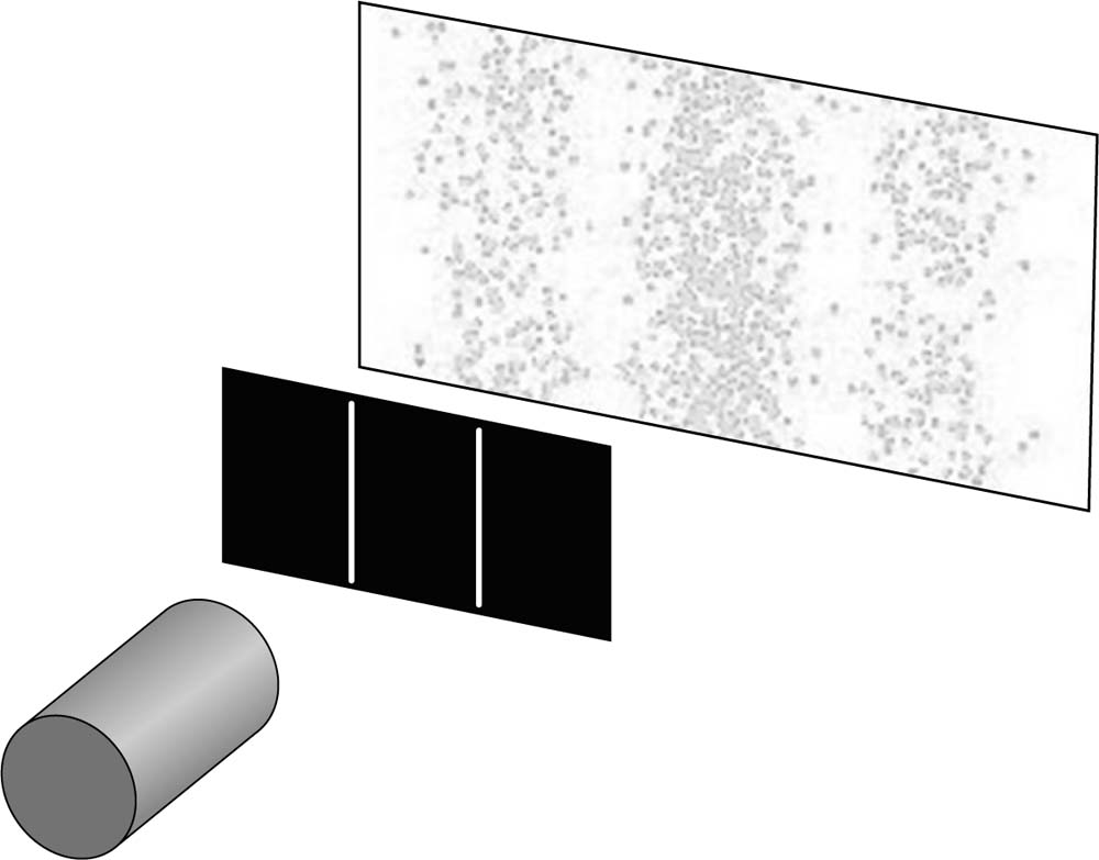
Fig. 7.3 The interference pattern after 3,500 photons have been detected at the screen (for the same slit separation and wavelength settings - note that altering these can alter the spacings between the bands). Is it a particle? Is it a wave? No, it’s neither (or both)!

Let us apply the language of wavefunctions to this setup. Remember from Chapter 2 that to each state of a system there is associated a wave-function ψ. From this we draw a probability P for being found to possess some particular property (e.g. to be at a particular location x on a screen). Let ψ(x) be the probability amplitude (a complex number) for the probability (which as an amplitude can be either positive or negative) of a particle in the two slit setup to hit the screen at a distance x from the center of the screen (where the center is the point lying equidistantly between the two slits). |ψ(x)|² is then the probability density whose integral over some interval gives the probability for finding the particle in that interval. In the case of the two slit experiment we clearly have two options (two mutually exclusive routes): ‘the particle goes through slit 1 to get to a point x on the screen,’ or ‘the particle goes through slit 2 to get to a point x on the screen.’ Represent these two possibilities by the amplitudes ψ₁(x) and ψ₂(x) respectively (associated with probabilities P₁ and P₂ respectively). The probability density for the particle to make a click at x is then:

P₁₂(x) = |ψ₁(x) + ψ₂(x)|².(7.1)

The density function will be peaked on x = 0 (directly between the two slits on the screen) and also on integer multiples of x = ±λD/s (where s is the slit separation, D is the distance between the slits and the detection screen, and λ is the wavelength of the beam).

Feynman’s remark about there being no classical explanation for this stems from the fact that a classical explanation would involve the simple additivity of probabilities of a particle going through slit 1 and a particle going through slit 2. In other words, for a classical particle theory we would have the sum:

P₁₂(x) = P₁ + P₂.(7.2)

That is, there is no interference between the alternative possible outcomes (represented by ψ₁(x) ψ₂(x)): we just have to add together the (classical) probabilities for the separate events, here P₁ and P₂, which would give a distribution peaked at x = 0 again, but decaying more or less uniformly as |x| > 0 (and we move away from the center) rather than displaying the peaks and troughs characteristic of wavelike phenomena and interference, as we see in Young’s diagram. By contrast the non-additivity of events for quantum particles is precisely what one expects of a wave. We must ‘supplement’ the classical probabilities with additional interference terms:

P₁₂(x) = P₁(x) + P₂(x) + I₁₂(x)(7.3)

As we saw in §5.3, there is a variety of options when it comes to interpreting probabilities, so there remains a question mark over how we should interpret these quantum probabilities: are they objective or subjective - i.e. about the state of the world or the state of our knowledge of the world? Are they about a whole bunch of similarly prepared events (relative frequencies) or are they about individual events (propensities or something of that sort)? Depending on how one thinks about these probabilities (objective versus subjective, or ontological versus epistemic to use an alternative terminology) one is faced with the view that quantum mechanics is either complete (so there is a fundamental limit to what we can know about the world: it is fundamentally probabilistic) or it is incomplete (so that there is perhaps some deeper theory that can explain and predict the funny behavior in the two slit scenario: there are ‘hidden variables’ that quantum mechanics misses). The same applies to the quantum states themselves, of course: since this is our central object of interpretation, either quantum theory is about world-stuff or knowledge-stuff.

So: the double slit experiment is closely related to one of the first conceptual questions to be asked about quantum mechanics: whether the wave-function gives a complete picture of reality or whether it is a step on the way to a deeper theory not subject to irreducible probabilities. If this is so, then what is the representation relation between ψ and the world? According to Einstein’s ‘ensemble interpretation’ it doesn’t in fact refer directly to the actual world at all, but rather to a non-existent distribution of many systems of the same kind. This is in order to make sense of the quantum statistics. We turn to Einstein’s famous argument in which he attempts to establish the incompleteness of quantum mechanics in §7.3. First we turn to the nature of probability and uncertainty in quantum mechanics.

7.2 Uncertainty and Quantum Probability

We have already met probabilities in physics in the previous chapter. However, in that case they were understood in an epistemic sense: probability was simply ignorance of the true facts. In situations in which the “true facts” are hard to determine, because of the extreme complexity of the system, for example, a statistical approach is a natural step. But the usage of probability is a matter of convenience. If only we had enough computing power to track and predict the movements of the parts of a complex system, and the resolving power to figure out their instantaneous states, then we could, in principle, eliminate probabilities and speak purely in terms of certainties. Weather prediction, for example, is (as you well know) fraught with uncertainty. But we do not think of this uncertainty as a brute fact about the world. Rather, we think that we simply don’t know (1) the initial conditions well enough to make certain inferences from them; (2) the laws well enough to feel confident about plugging in initial conditions (even if we did have them, since they are highly non-linear); and (3) we don’t have computers capable of running the evolution to make precise (unique) predictions. Again, probability here reflects our ignorance, rather than the world’s inherent indefiniteness. A 65 percent chance of rain tomorrow does not mean that the world is in a fuzzy state: we are in a fuzzy state!

In terms of the modeling of probabilities in such cases, we would think of them as measures over a state space in which those states are assumed to be uniquely mapped to definite physical states. The uncertainty is a measure of ignorance, rather than a measure of an objective feature of the world. In the case of quantum mechanics the ‘uncertainty principle’ is taken to express a more fundamental kind of uncertainty: there is a limit, integral to the laws of physics, according to which, for certain pairs of properties, we cannot know the values of both simultaneously with perfect precision.

A useful way of thinking about the uncertainty relations is in terms of the properties of the wavefunction as one switches between a well-localized position on the one hand and a definite momentum on the other. In the former case, the wavefunction is peaked at some point of space, with the momentum spread out. In the latter case, the wavefunction becomes a plane wave spread over the whole of space (in theory, out to infinity). Moreover, we can see that trying to localize a particle restricts its motion, which in quantum theory involves more energy: probing smaller scales demands greater energies, which is why ever larger particle accelerators are required to go to ‘deeper’ levels of reality.

However, the problem is that this switching is a function of whether a measurement is performed to determine the particular property. Born’s statistical interpretation, designed to make some sense of this switching, contains this same intrusion of measurement. The squares of the amplitudes were taken to correspond to the probability of observing some value of the relevant physical quantity given some measurement designed to determine it. The apparently bizarre wave packet, spread out over space, is not ‘really’ a physical entity, but instead represents probabilities for localized, observable events. However, as we saw in our discussion of the double slit experiment, these probabilities are rather unusual in that they involve interference between the various localized alternatives.

Mathematically speaking, the uncertainty relations rest on the fact that position x and momentum p provide dual (physically equivalent though formally inequivalent) representations of a quantum system’s state. They are related by a Fourier transform, which involves a reciprocal (inverse) relationship between the two representations: as the position amplitude (x isnarrowed down, the momentum amplitude (p) is spread (and vice versa). The uncertainty principle converts this mathematical result into a statement about our ability to gain information about a system’s ‘complementary’ observables (i.e. observables standing in just such reciprocal relations: those that are canonically conjugate):

∆x·∆p ≥ ħ/2(7.4)

Here ∆x and ∆p are simply the standard deviations (i.e. root mean squared) for particle position and momentum. In terms of joint knowledge then, if our grip on x is given by ∆x, then our grip on ∆p cannot be less uncertain than h/2 ∆x. In the extreme case ∆x = 0, our knowledge of ∆p is infinitesimally small (infinitely large uncertainty).

As mentioned, in quantum mechanics, if you want to know what is happening at smaller and smaller distances, then you have to increase the energy of the probe. Again, this is why the current generation of particle accelerators are so much larger than previous generations. Thinking in terms of using light to see smaller and smaller objects, this would simply mean that one needs shorter wavelength λ (higher frequency ν) light to uncover ever smaller objects. We can relate this wavelength to the momentum p as follows:

(7.5)

This inverse relationship (larger momentum implies shorter wavelength) parallels the uncertainty principle. To pin down an electron’s position with light we would have to use a short-wavelength/high-momentum beam. Of course, wavelength determines a natural limit on what can be resolved: no features smaller than the wavelength can be discerned. The problem is, if we use high-momentum photons, as we must to find out the position with a high degree of accuracy, then we kick the electron with those photons, imparting an uncertainty in its momentum. But if we were to use photons with lower momenta, then one faces the problem that the position is not pinned down closely enough.

Thus, this reciprocal relationship between distance and energy scales parallels the famous uncertainty relations in quantum mechanics, and indeed Heisenberg attempted to prove the uncertainty relations using ‘physical’ arguments based on such reasoning - he envisaged a fictional microscope that fired gamma rays at the particle. Quite simply, to localize a particle requires bouncing something off it. Finer localization requires higher energies so that the bounce will be stronger. However, this bounce will cause the particle to be uncertain in its momentum values, essentially being nudged to new values from the imparted momentum.

According to Heisenberg, then, a physically motivated interpretation of the relations could be given, based on the notion of a disturbance effect caused by measurement interactions. In order to determine the value of some quantity, one has to do something to it, and this changes its state. For example, to determine the position of an object we might naturally try to localize it using sound, light, or some other form of radiation. Heisenberg himself originally used this argument to prop up an epistemic view of uncertainty: it is our limitations that forbid us from finding precise values of conjugate pairs, but this does not imply that such pairs do not have precise values. However, swept up in Bohr’s interpretation, he succumbed to an ontological reading according to which there is no fact of the matter about the precise values: the values don’t exist. Indeed, without some interactions between the system of interest and a measurement device, one must remain silent about that system. Hence, the uncertainty relations in Heisenberg’s hands grew out of a wider philosophical stance concerning the meaning of physical statements: such statements must be associated with their means of being measured or bringing them about.

Einstein sought to produce counterexamples to this radical position (which he viewed as a denial of objectivity) by devising scenarios in which both quantities of a conjugate pair could have their values simultaneously pinned down in a way that defeated the uncertainty relations, much as Maxwell had attempted to beat the second law with his demon. However, Bohr is widely agreed to have gotten the upper hand. Another serious problem here is how to square the view that the wavefunction is a representation of knowledge with the very real phenomena that one finds in the slit and interferometry experiments.

Note that Bohmian mechanics faces no such issues over particle uncertainty since it essentially ‘buys’ definite positions for the particle using a nonlocal field, which ‘guides’ them (this approach is sometimes known as ‘the pilot-wave’ interpretation): hence, we have a hidden variables approach here, but a nonlocal one. Wave-particle duality is thus split apart into a particle, that is a particle at all times, and a wave, that is a wave at all times. Given this, the uncertainty relations are captured entirely by a ‘disturbance view’ rather than the uncertainty being a fundamental feature of the world.

There have been some recent experimental attacks on the measurement disturbance view of the uncertainty relations using ‘weak measurement’ (i.e. measurements that don’t collapse the state onto its eigenvectors, so that an initial state is kept intact: an interference pattern would still be observed on a screen following a weak measurement, for example).2 The idea is to measure some individual system state (such as the polarization of a single photon) but also measure how much the measurement disturbs the state. By doing a weak measurement prior to another measurement, the effect of measurement’s kick can be determined (by making a third strong measurement of the first property weakly measured). The results in the experiments conducted so far have found less impact than Heisenberg predicted: measurement disturbance, according to these results, does not add much to the inbuilt uncertainty of quantum mechanics. Whether loopholes can be found or not (e.g. in the assumptions of weak measurements, and whether they in fact constitute measurement in a strong enough sense), it does show that what seemed to be a purely interpretative distinction (the extent to which uncertainty is an artefact of measurement or a feature of the world) can, in principle, be linked to experiment, thanks to a new tool.

7.3 EPR, Odd Socks, and No-Go Theorems

In terms of philosophy of physics, 1935 was a good year: the famous EPR experiment (where E = Einstein, P = Podolsky, and R = Rosen) was presented, along with Bohr’s rebuttal, and also Schrödinger’s discussion, which involved the first proper discussion of quantum entanglement. EPR was Einstein’s grand challenge to Bohr’s Copenhagen (‘tranquilizing’) philosophy. The core of the debate was over whether quantum mechanics could be viewed as a complete theory (Bohr’s view), or whether it was fundamentally incomplete (Einstein’s view).

At the root of the historical argument between Bohr (and others) and Einstein was the issue of realism (or, better, ‘objectivity’): do the properties of objects have values independently of our observing them? In the early days, as seen in the previous section, it was supposed that there was a ‘disturbance’ triggered by a measurement that ‘brought the value into being.’ In other words, the very act of observation was something special. That is, observation generates or produces the values we observe in measurements: those values weren’t realized in the system (were ‘indefinite’) before the measurement (unless the system had been expressly prepared in such a value by prior measurement). It was this feature that so disturbed Einstein - and not the statistical nature of the theory, as is often supposed (encapsulated in his ‘God does not play dice’ remark). One might quite reasonably side with Einstein on this: it does seem rather strange to think that the world does not have its properties given independently of our interactions (that ‘the Moon is not there when nobody looks,’ as he once put it to Bohr).

What also concerned Einstein was the apparent ‘spookiness’ of the interactions that would happen in distantly separated regions of space if quantum mechanics was supposed to provide a complete representation of reality. Locality was paramount: after all, it had been the central principle of both of his relativity theories in that action at a distance was explicitly ruled out. The notion of an objective reality is linked to this: the values an object has should not be linked to values had by another causally isolated system.

A real state (commonly called ‘an ontic state’ in modern discussions) is simply one that exists independently of our measuring it or knowing about it (an ‘element of reality’ in Einstein’s terminology): it is objectively given in the sense that there is a fact of the matter about which values are exemplified at all times. If we measure such a state then we will be finding out what its state was (assuming there is no disturbance) beforehand. The states of a classical mechanical system can clearly be thought of in this way, as revealed by measurement. For example, in a Hamiltonian setting (the classical mechanics in phase space, from §2.2) our (instantaneous) states will be phase points x = (q(t), p(t)), which will determine unique trajectories. Any intrusion of probability here is associated with ignorance, in principle eradicable by supplying the additional information: let’s do the same with quantum probabilities, says Einstein. Assume that the states of quantum mechanics could be filled in by hidden variables.

The so-called Kochen-Specker theorem already causes serious problems for the idea that quantum objects possess their properties in a simple ‘common-sense’ way, as suggested by such Einstein-style incompleteness claims. This conception of quantum properties is known as ‘value definiteness’: observables on quantum mechanical systems have definite values at all times, not just when measured. However, given an assumption of non-contextuality (that properties are possessed independently of which measurement we decide to perform), the Kochen-Specker theorem shows that the job of definite value assignments to all properties simply cannot be carried out. This is essentially a formal result having to do with the way observables are represented by Hilbert space operators in quantum mechanics. However, let’s put the Kochen-Specker theorem aside and focus on the famous ‘EPR experiment,’ since this leads us to matters of entanglement and nonlocality.

Einstein famously defended ‘local realism’ (against quantum mechanics) in his debate with Bohr. This consists of two distinct components:

1. Physical systems have properties independently of our observing them [they have objective reality]

2. Physical systems that are ‘spacelike separated’ (with one lying outside of the other’s light cone) cannot causally influence one another so that measurements on one affect measurements on the other [= principle of locality]

EPR tended to focus on position and momentum values, given the historical context fixed by Heisenberg’s uncertainty relations. But let’s see how their argument is supposed to work by looking at David Bohm’s simpler version involving spin measurements (known as an EPRB experiment). Here we have a central source that generates a pair of particles, A and B, in what is called a spin-0 (singlet) state (where means that particle A is spin up and particle B is spin down, so that the total spin cancels to zero: the symbol ⊗ refers to the tensor product used to combine several subsystems in quantum mechanics). Formally, we can write the resulting state for the experiment as follows:

(7.6)

This is an entangled state: we can’t express the state in terms of separate, well-localized states at the detectors, since the singlet state doesn’t ‘factorize’ in the sense that the total wavefunction (representing the state of the system as a whole) cannot be expressed as a combination (tensor product) of the states of the parts. The particles are sent out to the left and right, to have their spin-components measured at detectors that lie at spacelike separation to one another (see fig. 7.4) - this is, of course, to implement the locality condition. The measured spins will always be perfectly anti-correlated because of the conservation of angular momentum: if the left particle is measured to have +ħ/2 then the right will always be measured to have −ħ/2 (and vice versa). Indeed, the choice of which direction to orient the detector is made once the particles are sufficiently separated to let the locality principle really get a foothold - since these orientations are chosen ‘at a whim’ (a ‘free will’ assumption), the particles cannot have conspired to set their values so as to establish their perfect correlations.

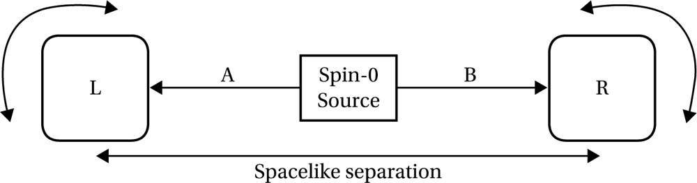
Fig. 7.4 A pair of particles in an ‘EPR state’ (a spin-0, singlet) is sent out to spacelike separation to be measured by a pair of reorientable spin-measurement devices (for the z component of spin). The direction of spin measured is chosen at each detector only once the particles are separated sufficiently to avoid any ‘conspiring’ to generate correlated results through direct communication (i.e. by local action or signaling).

The idea of EPR is then to compare ‘common-sense’ (as given by the locality and realism assumptions above, leading us to think that any measured correlations must be due to states had before measurements were made) with quantum mechanical predictions concerning the correlations we would find if we generated data on many such spin measurements. EPR claim that quantum mechanics fails the common-sense test by requiring nonlocal action (entanglement across spacelike separated distances). The common-sense view would simply point to the common origin in which the spin was zero, and so must be conserved. There would be perfect anticorrelation even when a free choice is made to alter the direction of the detector, rotating it by some amount - the spin-0 state has rotational symmetry, so it is impervious to such changes. A measurement will ‘project’ the state onto either depending on whether particle A is measured to be spin up or down respectively. The problem raised by EPR is: how on Earth do the particles know what the other particle will ‘reveal’ on measurement so that it can coordinate itself accordingly? We can’t run the classical ‘common source’ scenario in this case because that requires that the state would have been in an ‘eigenstate’ (think of this as a definite value for the measured property) all along from the source to the measurement so that it determines the measured result: but our singlet state is not of this kind. Worse, we have the freedom to choose our measurement direction (e.g. x-component instead of z) in mid-flight, while still preserving the perfect anti-correlated results - classically this would require that the information is built-in to the particles at the birth for all possible spin-measurements (including those that don’t commute and so face the Heisenberg uncertainty relations). Again: how do the particles know what to do?

According to EPR there are just two possible explanations: (1) superluminal messaging allowing measured states to be communicated at an instant between particles, or (2) there is something missing from the quantum description of state, and this extra something is what determines the (anti-)correlations. Since the first option involves spacelike separated events, however, it seems that the measurement and subsegment distant effect could be switched by choosing an appropriate frame of reference, so that the link is not a Lorentz invariant notion.

As John Bell showed many years later (and as we see in a moment), it is possible to generate an experimentally testable difference between the common-sense (hidden variables) and quantum explanations: quantum mechanics will make different predictions to such a locally realistic theory. Let us just step back for a moment to consider an example of Bell’s that makes the common-sense (classical) idea seem especially appealing.

The Irish physicist John Bell is often looked upon as an oracle by philosophers of physics, and not without justification: he is responsible for transforming the foundations of physics in such a way that philosophers of physics are likely never to be short of tasks. It is widely acknowledged that Bell’s theorem, from his paper on the EPR paradox, was a much needed shot in the arm for foundational research on physics. It has been labeled ‘experimental metaphysics’ since it seems to rule out a metaphysical stance (Einstein’s notion of ‘local realism’) - it was Alain Aspect who first realized that Bell’s thought experiment could be made flesh, devoting his PhD thesis to the subject (though he performed it with photons and polarizers, with calcium atoms as the source).

Bell distinguished between observables, which we have met, and ‘beables’ (that is be-ables). The latter are supposed to be distinct from matters of observation and measurement: a system’s beables constitute the values that it has rather than what it will have when it is observed. The old orthodox interpretation of quantum mechanics had it that the theory was all about what would be observed upon measurement, not about what was before measurement. In other words, measurements are not taken to reveal the pre-existing values of the measured particles, but in some curious way they ‘bring about’ such values. The famous EPR argument rests on just this distinction, with EPR taking the view that a sensible theory must be about beables, and Bohr (and followers) arguing that quantum theory, sensible or not, is about observables: things whose raison d’etre is to be measured.

In the case of EPR correlations, as we have seen, a natural response is that they are no more surprising than everyday correlations in which there is a past preparation making it the case that if one outcome is observed at one end of the experiment, another known outcome must be observed at the other regardless of the spatial distance that separates them at the time of measurement of either. Bell makes this intuition very clear with his story of Reinhold Bertlmann and his eccentric practice of always wearing odd socks:

Dr. Bertlmann likes to wear two socks of different colors. Which color he will have on a given foot on a given day is quite unpredictable. But when you see that the first sock is pink you can be already sure that the second sock will not be pink. Observation of the first, and experience of Bertlmann, gives immediate information about the second. There is no accounting for tastes, but apart from that there is no mystery here.

We can even suppose that Bertlmann bundles together socks of distinct colors in his sock drawer at home, randomly grabbing a pair each day. The analogy with quantum particles and their properties looks fairly direct. In this case we suppose that a pair of particles is prepared in a singlet spin state, in which they are described by a single wavefunction in which the particles’ spin-values are opposed to one another: if one is definitely spin-up the other is definitely spin-down. They are sent apart to enter a pair of widely separated Stern-Gerlach experiments (used to determine their spins along some given axis) whose magnets will either result either in the particle’s going upwards or downwards (the Bohm version of EPR just mentioned).3 Which will happen for any given individual experiment is only known with a certain probability, but one can say with certainty that if one value is found at one experiment then the opposite will be found at the other. One could, if so inclined, describe Bertlmann’s socks by a wavefunction, and even speak of it as ‘collapsing’ when we notice the color of one of his socks (so that the composite state featuring both socks is fully known).

Of course, in the case of Bertlmann’s socks one does not say that observing a pink sock on one of his feet causes the other sock to dramatically alter its ontological status to non-pink. We do not collapse his sock from a fuzzy to a definite state. The only thing that was fuzzy was our knowledge. Any assignment of uncertainty about sock color (represented in the wavefunction) is entirely epistemic.

The question is: what of the situation with quantum particles? Can we adopt this same epistemic strategy with them, so that the experiments are simply detecting (or revealing) the properties of the particles that they had all along? After all, isn’t that what experiments are for: finding out what value some system had?

This is where Bell’s famous no-go theorem enters.4 It provides a criterion for deciding whether the correlations in your theory are like Bertlmann’s socks or not. It also provides a route for testing whether our world is a Bertlmann-world or something more puzzling. Or, to put it Bell’s way, we need to find a way of deciding whether quantum mechanics is local or nonlocal, and then we can figure out whether the world itself is home to nonlocal influences or not.

Firstly, we need to get a clearer grip on the central terms of the debate.

· Einstein Locality: this applies to multi-part systems in which the system’s parts are spacelike separated. Then for some joint operator that is built as a product of the parts’ individual operators (a superposition of the separate parts’ states), its value will be built from the individual parts’ values in the same way. The values of the individual components are independent from one another in the sense that a measurement of one does not interfere with the other.

The notion of a ‘correlation’ too should perhaps be spelled out. We know from the news that there are often stories pointing out a newly discovered link between some substance and a health condition. These provide us with various pairings: ‘smoking and lung cancer;’ ‘coffee and Parkinson’s disease;’ ‘marijuana and schizophrenia;’ and so on. These are correlations rather than causation because the exact mechanism is not known: it is a statistical link. One might have found from some study that a large proportion of people who smoked a certain amount of marijuana also developed schizophrenia - more so than the general ‘background rate’ of schizophrenia in the population. So we could then assert that the probability of having schizophrenia given that you smoke marijuana is greater than if you didn’t. But, so the saying goes, correlation does not equal causation. For example, it is possible that people who develop schizophrenia are more likely to self-medicate to alleviate the anxiety of stigmatization, so that the direction of influence is reversed (schizophrenia causes smoking, rather than the other way around).

A correlation once discovered is often a first step in filling in a deeper causal story, or in showing how some statistical error is confounding the true results. Hence, there is a task of explaining or explaining away a correlation once one has been found to occur in nature. There might be a variety of things leading to the presence of a correlation. There might be genuine causation going on, replete with a mechanism linking the two variables. For example, one might discover a gene that some people have that is ‘switched on’ by the some specific component contained in marijuana smoke. Unless one does lots of studies to reveal the generality of the correlation it might have been a simple coincidence that in this population studied there happened to have been more schizophrenics than would ordinarily be expected. I already mentioned above the idea that the schizophrenia might be leading to smoking as a form of self-medication. In this case we could seek some deeper brain disorder that would be responsible for both variables, thus providing a common cause. (The standard example of the notion of a common cause is in explaining the correlation between yellowing of the fingers and lung cancer. There is such a correlation, but neither causes the other: smoking cigarettes causes both. Philosophers speak of the common cause as ‘screening off’ the original correlation: smoking causally screens yellow fingers from lung cancer.) What we had initially would then be a ‘causally spurious correlation.’

A final option is that the correlation is simply ‘brute’: an inexplicable feature of the world that cannot be further analyzed. This is, scientifically speaking, not the kind of thing we would wish for. However, as we will see, the correlations of certain quantum mechanical experiments are seen to be just like this according to many interpretations. The word ‘correlations’ should immediately indicate that we are dealing with statistics here: results of many experimental runs.

The correlations here are remarkably simple: if a particle is found to be spin-up on one side, then it will be found to be spin-down on the other side regardless of how we establish the magnets’ orientations (so long as these orientations are set the same on both sides, anywhere between 0 and 360 degrees, the θ value: generally chosen to be a multiple of 120 degrees, so that there are three possible settings).

As mentioned already, a natural (common sense = Bertlmann’s socks) response is that the particles were forged at the same source, and ‘simply carry their instructions around with them.’ These instructions (hidden variables) reveal themselves when measured and are responsible for what is measured. If we performed lots of experiments to determine this, we would find a distinctive set of results appearing: if there were no correlations, as we would expect given the large spatial separation forbidding direct causal interaction, then we would find that the joint probability distribution would factorize into a pair of individual probabilities for the experimental variables.

Take some general pair of outcomes A and B (which might be our spin up and down results), and take some adjustable setting values, a and b, that will determine what measurement is carried out on A and B respectively. Our concern is with the joint conditional probability distribution: P(A, B|a, b) - the probability of getting outcomes A and B given (i.e. conditional upon) the settings a and b. If this does not factorize into independent probabilities, then we have a correlation: P(A, B|a, b) ≠ P₁(A|a)P₂(B|b). Common sense tells us to look for some causal reason for correlations. Think of yellowing fingers and lung cancer (a standard example). We find that P(A, B) ≠ P₁(A)P₂(B). Why? It doesn’t seem that one can directly cause the other: no mechanism seems to link them. The trick is to add additional causal factors, a and b, so that we condition on whether those with lung cancer and those with yellowing fingers are also smokers. There might well be a few other factors, λ, such as genetic disposition to smoke, that further ‘causally unlink’ the yellowing and the lung cancer, tracing both back to some common origins. When we take these into consideration, we will find a joint probability distribution that factorizes:

P(A, B|a, b, λ) = P₁(A|a, λ)P₂(B|b, λ)(7.7)

The ‘settings’ a and b are assumed to be independent: Bob’s smoking in Kansas is not a likely cause of Vic’s smoking in Kazakstan. So the EPR/hidden variables idea goes. The λ in this case will be some, as yet undetermined, causal factors (the hidden variables) that when supplemented into our model of the EPRB experiment will explain the correlations without utilizing any spooky influences - they can potentially take many forms. The a and b are the freely chosen settings for the detector orientation; as with the Vic and Bob’s smoking, these must be assumed independent (known as ‘parameter’ or ‘setting independence’) lest action-at-a-distance type influences enter the picture. This is in stark violation of special relativity. The similar independence of the outcomes (outcome independence), however, is not thought to be in violation of relativity. The difference is in the ability to control the parameters a and b (e.g. to signal), but not in the case of A and B (note that I am speaking of the outcomes and the experimental wings by A and B here). To sum up: a hidden variables model will say that the outcomes A must only depend on a and λ, not on the goings on with the b-settings. Fiddling with b should alter nothing about A, and at A we have no knowledge of these fiddlings due to parameter independence (implementing locality). Bell’s theorem tells us that one of these independence conditions must be false.

We know also that if we consider −z (or a 180-degree) rotation of the detector, then the two outcomes will then be perfectly correlated: anti-correlated for 0; correlated for 180. That leaves a whole lot of orientation settings that can be utilized independently at the two sides of the experiment. Hence, if we only focus on measurements made with the same a and b settings then we expect the outcomes to be (anti-)correlated, and there is no scope for distinguishing quantum and hidden variable models: we know that the probability of getting the same outcome is zero since we have a singlet state with opposite spins demanded. The interesting divergences come from considering general settings. Indeed, it is found that divergences in predictions occur when the relative angle between the settings differ from 0 and 180 (and also 90 and 270). The respective predicted correlations for hidden variables and quantum models are shown in fig. 7.5.

These correlations can be used to generate inequalities for the degree of correlation such that if the world has hidden variables, then the degree of correlation will be greater than or equal to some value, for example.

This graph (in fig. 7.5) also reveals that the predictions of a quantum model cannot be replicated by a (local) hidden variables model. The incompatibility provides the basis for an experimental test: each model will make a set of distinct predictions that will enable us to test whether our own world is quantum (non-local) or not. Quantum models will violate a feature (Bell’s inequality) that a local, classical model will satisfy.

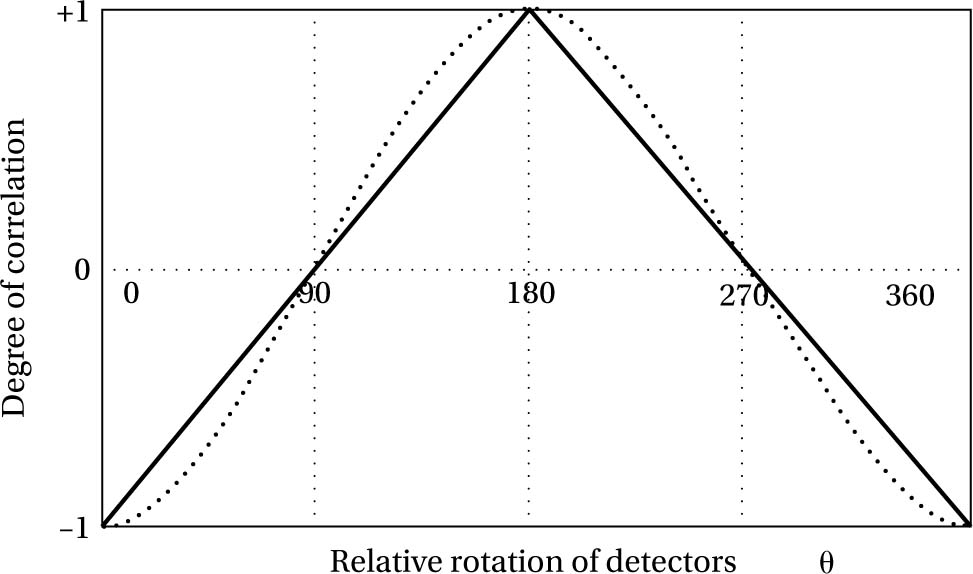
Fig. 7.5 The degree of correlation predicted by a hidden variables model (solid line) and a quantum mechanical model (dotted line) for various relatively rotated detector settings. Though there is agreement at multiples of 90 degrees, there is divergence elsewhere.

Experiments performed by Alain Aspect and others have since confirmed quantum mechanics over Einstein’s hidden variables view of how the world should be. This leaves either or both of the two components of local realism at odds with the world. Either could in principle be denied. In the case of objectivity, one would have to give up on the idea that physics is about ‘the way the world really is’ (Bohr’s view). In the latter case, one must accept the existence of superluminal connections: nonlocality. However, nonlocality in this case is rather different from nonlocal signaling, and the concept must be treated with care. Certain prohibitions elsewhere in quantum mechanics forbid the use of nonlocality as a means of superluminal communication.

There is some controversy over the validity of the results, and these work by finding flaws in some assumption of Bell’s proof. One possibility, considered by Bell himself, is that the free choice of the experimenter is an illusion, so that the universe determines which settings will be selected. The universe thus orchestrates the correlations by determining what the experimenters decide to do (superdeterminism!). Here one must weigh up the relative implausibilities of nonlocality versus superdeterminism…

There is a related philosophical puzzle of how we are to interpret entangled systems ontologically speaking: what kind of world is a world containing entanglement. Lenny Susskind calls entanglement “the essential fact of quantum mechanics” (see p. xi of his book listed in Further Readings): it’s what separates quantum from classical phenomena. Schrödinger, who coined the term in a 1935 paper, agreed:

When two systems, of which we know the states by their respective representatives, enter into temporary physical interaction due to known forces between them, and when after a time of mutual influence the systems separate again, then they can no longer be described in the same way as before, viz. by endowing each of them with a representative of its own. I would not call that one but rather the characteristic trait of quantum mechanics, the one that enforces its entire departure from classical lines of thought. By the interaction the two representatives [the quantum states] have become entangled. ([44], p. 555)

Entangled states, remember, refer to many particles (a composite system) that are in an eigenstate of some observable in a joint sense (as a pair), but not individually. For example, in the case of a spin observable, we might know that the total, joint system has spin 0, but not be any the wiser about the spins of the particles themselves, which can be measured up or down (+ or −ħ/2). However, as we have already seen, we can say that if a measurement yields spin up on one particle (for some measurement orientation), then the other particle is spin down (for the same measurement orientation). The non-factorizability appears to lead to a kind of ‘holism’ since ontological independence of the systems can’t be established - though a measurement will ‘disentangle’ them according to many interpretations. Here’s Schrödinger again:

Another way of expressing the peculiar situation is: the best possible knowledge of a whole does not necessarily include the best possible knowledge of all its parts, even though they may be entirely separate and therefore virtually capable of being the ‘best possibly known,’ i.e. of possessing, each of them, a representative of its own. The lack of knowledge is by no means due to the interaction being insufficiently known - at least not in the way that it could possibly be known more completely - it is due to the interaction itself. Attention has recently been called to the obvious but very disconcerting fact that even though we restrict the disentangling measurements to one system, the representative obtained for the other system is by no means independent of the particular choice of observations which we select for that purpose and which by the way are entirely arbitrary. It is rather discomforting that the theory should allow a system to be steered or piloted into one or the other type of state at the experimenter’s mercy in spite of his having no access to it. ([44], p. 555)

In other words, we are free to choose, arbitrarily, which measurement to perform on one of the separated particles, but the disentangling will still occur for both particles regardless of their spatial separation. One spanner in the works for large spatial separations is that special relativity becomes relevant: this impacts on the total wavefunction for the system, which becomes non-factorizable (thus deepening the appearance of holism). However, at the same time the macroscopic distances involved in situations in which relativistic effects play a role make it hard to retain the coherence of the quantum state.

Though we see Schrödinger grappling with entanglement, and some of its odder implications (such as quantum steering and holism), it was left largely untouched until John Bell’s work on the subject three decades later. Schrödinger himself thought that the nonlocality was unphysical. The past two decades or so have seen a radical transformation in the way entanglement is understood. Once viewed as a mysterious ‘spooky’ phenomenon, it now forms the basis of experiments and quantum mechanics. In more recent times, entanglement is so commonplace that computer scientists speak of it as a ‘resource’ to be manipulated and optimized.

Given the existence of genuinely entangled states, an interpretive task emerges for philosophers of physics: what kinds of things are they? This has proven to be highly controversial territory, with some arguing that entangled states call for entirely new ways of thinking about the world’s ontology. Formally, remember, an entangled state (for an N-dimensional system) is ‘non-factorizable’ in the sense that a joint wavefunction for many particles cannot be written as separate wavefunctions for the subsystems: . Hence, there is a suggestion even in standard quantum mechanics that the world might not submit to being carved up in terms of ‘individual things.’ Entanglement involves the notion that the total quantum system is not reducible to the intrinsic properties of its subsystems, thus exhibiting a kind of ‘holism.’ Paul Teller developed a position known as ‘relational holism’ to capture this ‘whole is more than the sum of its parts’ aspect of quantum mechanics: the relations cannot be reduced to the non-relational properties of the relata (that is, they do not supervene on the non-relational properties on the relata). This aspect is known as ‘non-separability’: the inability to view the state of the world as reducible to local matters of fact.5 This amounts to a kind of emergence too, since the emergent properties are not definable in terms of the non-relational properties of the subsystem parts. Likewise, Michael Esfeld and Vincent Lam [11] have argued that such relations in entangled systems can be understood as simply unreducible to the intrinsic subsystem properties. Ultimately, they propose that the ‘object-property’ distinction (where ‘property’ includes relations and structure) is not a fundamental ontological one, but a conceptual one. Hence, the phenomenon of entanglement links directly to deep matters of ontology and metaphysics.

7.4 The Quantum Mechanics of Cats

In a very tiny nutshell, the quantum measurement problem can be summed up as: quantum mechanics seems to allow superpositions to be amplified up to the macroscopic level. We don’t see such superpositions of macroscopic alternatives. Therefore, we either need to find a way of burying them where they cannot be experienced or explain why they are not experienced in some way consistent with quantum theory (and thereby solve the measurement problem), or else reject the theory.

One might easily be forgiven for thinking, on the basis of much of the literature, that the quantum measurement problem is the only philosophical problem facing quantum mechanics. Its tendrils spread into many other areas in the conceptual foundations of quantum mechanics. The measurement problem follows quite simply from apparent facts of experience (the ‘definiteness’ of measured or observed properties) together with the assumptions of:

Linearity: time evolution under the Schrödinger equation is linear so that superpositions can ‘spread’ through interactions, so that if one system is in a superposition of its possible states, any system it interacts with will also evolve into a superposition of states;

Universality: the wavefunction ψ is able to describe any and all dynamical systems in nature.

With these two properties given we can infer that macroscopic objects will, like their microscopic cousins, be governed by quantum mechanics. This means that they too must have a linear state space, and so behave in a wave-like manner. This, in turn, means that we can have states such as (here we go!) a cat that is a linear superposition of both alive and dead (or neither alive nor dead) states. Such (macroscopic) states are, of course, never observed in nature. Rather, we observe outcomes: specific, unique, individual events: one or the other. Hence, we have a dilemma: (1) either our ideas about macroscopic objects are wrong; or (2) QM is false; breaks down at the level of macroscopic objects (such as a system capable of observing); or needs modifying in some way. This has some resemblance between the problems faced by the statistical view of entropy, with the conflict between theory and observation there: theory predicted a high entropy to the past as well as the future, but we observe this feature only in one direction. Similar mind-stretching (to Boltzmann’s cosmological/ Anthropic ideas) results in the context of the measurement problem in the attempt to resolve it.

This duality (wave behavior versus particulate behavior) is at the root of the measurement problem. The wave behavior is described by Schrödinger’s equation. This is perfectly adequate for situations in which the system is not being observed or measured. However, seemingly, when it is measured a different kind of evolution occurs: a disruption of the linear, wave behavior. To give a simple example: suppose that we have some radioactive element that has a half-life of ten minutes. If we have a bunch of these atoms then after ten minutes have elapsed we can expect half to have decayed (into various decay products: radiation). If we consider a single such atom then after ten minutes if we don’t measure it (e.g. with a geiger counter), then the quantum mechanical behavior will see it evolve into a linear superposition of decayed and undecayed: 50/50. The geiger counter, however, will register a definite event: click or no click. This transition from superposition to individual event constitutes a second form of evolution in quantum dynamics - though not all agree that it is a genuine feature of reality. This 50/50, ‘blended’ behavior so far is applied to the world of the very small, and so, though conceptually problematic, poses no direct observational problems - note that the 50/50 distribution is not necessary for the argument, which requires that a superposition be formed in which it is not the case that one state has probability 1 while the other states have probability 0: this latter is the characteristic of a measured state (which is another way of stating the problem).

The infamous Schrödinger’s cat example makes use of this simple split in the kinds of evolution. The radioactive substance is coupled to some poisonous gas, both of which are within a closed box, such that if the substance decays then an unfortunate cat (also confined to the box) will perish. If it does not decay, then the cat is safe. However, we have seen that if a quantum system is not measured, it will enter a superposition of states, here: |decayed⟩ + |not decayed⟩. But the fact that the behavior of the atom is coupled to the poison implies that there will be an associated superposition of poison (prussic acid in Schrödinger’s original example!) | emitted) + |not emitted⟩. And, finally, since the cat’s continued existence depends on the poison, and in turn the atom, it too will enter a superposition of |perish⟩ + |safe⟩. In other words, a superposition at the microscopic level (not directly observable) is amplified (through the evolution of the basic dynamical law of quantum mechanics) into a macroscopic superposition (with no definite component realized).

This obviously contrasts with the fact that we know our experience when opening the box to see what happened will reveal an individual event (one or the other component of the superposition). There seems to be, then, a conflict between quantum mechanics and experience! Macroscopic superpositions are predicted by quantum mechanics; but our experience reveals no such thing. This is the quantum measurement paradox. It is also another kind of incompleteness result since quantum mechanics seems not to be able to tell us about the state in the box.

What is bizarre about this is that it is most often assumed that our experience (of macroscopic definiteness) is veridical (true to the facts of the world) so that if quantum mechanics is also true, then we are somehow affecting quantum states when we perform measurements. This is known as reduction of the wave packet by observation or measurement, or more formally as ‘the projection postulate.’ It is a solution alright, but requires filling in by some kind of mechanism to be satisfying. We mention a few of these here. The most famous (the one that ‘stuck’) is the Copenhagen interpretation.

According to the Copenhagen interpretation, the quantum state’s function is to provide information about measurement outcomes. Given some preparation of the system in some state, one can then plug this state into the dynamical equations of quantum mechanics to make (probabilistic) predictions about outcomes at later times.

At the root of Bohr’s understanding of quantum mechanics was the notion of complementarity. This refers to a pair of features or quantities that are both required to understand a system, yet cannot be measured or determined simultaneously. The best known complementary pair are position and momentum of one and the same particle. We saw this earlier: the more we try to pin down one, the less we are able to pin down the other. One could place a screen to detect the interference fringes (and so the wave-like aspects) in a double slit experiment (with no attempt to detect which slit a particle travels through); or one could position detectors at the slits, thus revealing the particle-like aspects. Doing either of these experiments rules out the other: they are mutually exclusive. One can go bonkers trying to figure out ways to evade this embargo and achieve precise determinations of both aspects - but that does not mean it is not a good exercise! The point is that although wave and particle aspects appear to be flatly contradictory, the embargo on simultaneous measurement means that it doesn’t cause us trouble: it’s wavy when we detect for wavy aspects and particulate when we detect for particulate aspects.

This latter feature points to a kind of relationism in Bohr’s interpretation. The exhibition of a property by a system is relative to a measurement designed to reveal it. What Bohr does not want to countenance is the notion that systems ‘just have’ properties regardless. This relativization is precisely what was behind Einstein’s refusal to accept Bohr’s approach, remarking that he believed the Moon was there even when nobody was looking (i.e. doing a position measurement). In the case of the cat, it does not have a definite state until a measurement is performed. A ‘classical’ measurement apparatus is needed to do this: a human eyeball, or a Geiger counter. It doesn’t matter so much about the size, but that it can provide an observable output is important.

Hence, in between measurements (when not aligned with some experimental arrangement), the system is described by a quantum state that represents a kind of disposition or potential to generate outcomes. To get the classical world out of quantum mechanics, one needs classical equipment to register the results. A meaningful situation, then, demands a system and an apparatus.

One of the most problematic aspects of the Copenhagen interpretation is the special status it assigns to measurement (and the classicality demanded to make sense of it). It almost looks as though the demand for classical measurement devices pulls the rug out from under quantum mechanics, rendering it non-fundamental and non-universal. Just what is so special about those processes we call measurements? This amounts to another form of the measurement problem, though one not grounded in the clash between theory and experience.

Eugene Wigner raised the following problem (known as ‘Wigner’s friend’) for the Copenhagen approach to the Schrödinger cat paradox: what happens if you put the scientist (initially observing the cat in the box) inside an even bigger box, which can be observed by another (exterior) scientist? Now the first scientist is part of the system rather than the measurement device. In this case, the scientist in the box is described by a quantum state, a superposition state (atom + poison + cat + scientist) until a measurement is made. The exterior scientist now has the power to collapse the wavefunction by peeking inside. In principle, of course, this boxing procedure could be carried out ad infinitum, producing a sequence of boxes each with their own scientist, like nested Matryoshka dolls, with the most exterior scientist always having the ultimate power to collapse the wavefunctions of those within, which are in an indefinite state until observed.

Wigner found this implication absurd, but proposed instead what strikes many as far more absurd: the mind causes quantum states to collapse. So whenever there is a mind, there will be the ability to collapse. Hence, contra Bohr, there is a limit (far smaller than the universe) to the ‘system versus apparatus’ split enforced by consciousness (awareness). A measurement result would seem, after all, to demand awareness of the meaning of the result. Perhaps the cat itself is aware enough to collapse wavefunctions? Such ‘mental’ intrusions (also espoused by von Neumann) were mercilessly mocked by Bell, who inquired as to what level of mind is needed to collapse a wavefunction: an amoeba or only someone with a PhD?! The problem with this solution, though it is intuitively obvious in a certain sense, is that it introduces another (perhaps deeper) puzzle: what is this mind stuff? How does it work its magic? Wigner has no account, and the solution dissolves into a supernatural speculation. It also leaves the difficult problem of all of that ‘pre-mind’ time out of which minds themselves must have emerged.

The reasoning in the Wigner’s friend example here is, however, perfectly correct, and it basically replays the original Schrödinger cat scenario at a meta-level. If the cat is dragged into the quantum superposition of the poison, which is itself dragged into the superposition of the radioactive substance, then any system that subsequently interacts with the cat (or some of its properties that it can become correlated with) will likewise be dragged into the superposition. This is a simple consequence of the linearity of the dynamics (the evolution described by the Schrödinger equation): superpositions ‘infect’ systems they come in contact with, like a superposition virus, forcing them into superpositions too. Except they clearly don’t, since we know perfectly well we would only ever see a definitely dead or definitely alive cat. Hence, Wigner’s (difficult) decision to let the buck stop at the observing mind.

Though clearly very distinct from the Copenhagen approach, Wigner’s proposal too relies on the notion of a primitive measurement process, capable of collapsing the wavefunction (and so destroying any interference that would allow us to see quantum superpositons of distinguishable alternatives). But measurement involves a coupling of physical systems and, unless you’re Wigner and believe in a dualist scheme (with mind and matter distinct), must also be governed by the same laws as any other physical interaction. So why does measurement play a special role? Surely it’s just physical systems interacting? Why isn’t it subject to a quantum description too?

A fairly standard view these days is that measurement is indeed ‘just another physical process,’ but in real cases of measurement there are some features that make it at least a little special. For one thing, measurement apparatuses are big: the detection events in the various experiments we’ve been discussing (the clicks on a scintillation screen in the two slit experiment; the large spatial separation between the beams of a Stern-Gerlach experiment, etc.) are decidedly macroscopic: they involve large numbers of particles that serve to amplify some microscopic event. We know that it is difficult to make large things exhibit quantum interference effects: one can hardly throw a team of scientists through a double slit experiment to build up a wavy interference pattern on a screen (you could never get the ethics approval anyway in these politically correct days)! We find that the large results that our detection equipment indicates are macroscopically distinguishable correlates of the micro-systems they are calibrated to measure.

The backbone of this ‘size matters’ idea leads us into what has become a standard part of modern quantum mechanics: decoherence. Decoherence has been viewed by some as a sort of magic bullet for the measurement problem, capable of explaining away the absence of interference effects in our observations, while being perfectly within the realm of the physical, and just an application of ordinary quantum mechanics (without projection or any of that funny mind stuff). Recall that the curious interference effects at the root of the double slit experiment and the measurement problem (and entanglement) come about from the existence of the quantum phase θ. If this can be reduced to zero somehow, then the curious phenomena disappear and the behavior looks classical. Decoherence is often touted as one route to the zeroing out of phase, and therefore interference, and therefore the measurement problem.

But it is not a complete miracle cure. The idea is that when interactions occur between a microscopic system (with very few degrees of freedom) and a measuring device (lots of degrees of freedom), we also need to take into account the fact that both are situated in a wider environment with a vast number of degrees of freedom, and evolving according to the (linear) Schrödinger equation with respect to this environment. This environment thus has the effect of ‘absorbing’ the quantum interference through correlations with these degrees of freedom. The measured system thus engages in a multitude of other interactions with air molecules, photons, and what not, in such a way that in focusing on the apparatus alone one would be forgiven for thinking that it is in a mixed state (i.e. with good old classical probabilities for the alternatives), with no interference (between the alternatives) present at all. In other words, ‘for all practical purposes’ one has gotten rid of the problem.

Measurement, in this case, can be viewed as converting a genuine superposition into what looks like a mixture (i.e. something that can be dealt with using classical probabilities). In different terms, it looks like an example of an irreversible process, where we have lost information about the superposition into the environment Φenv. But, as the above suggests, the superposition is still lurking in the world, spread throughout all of the degrees of freedom that are involved in any real physical measurement. The interference is still in the total state (Φenv ⊗ ψsys) but not in either of the ‘reduced’ states: Φenv or ψsys. To extract the information needed to exhibit the interference would perhaps require a Maxwellian demon, tracking all of the interactions, thus enabling reversibility. But in principle, the process is reversible.

This split between quantum and classical is very different from the shifty split of the Copenhagen school, where one moves it depending on context (i.e. on what the system is and what the apparatus is). The effect involved in decoherence is one that occurs by degrees, dependent on the number of degrees of freedom of the environment, rather than on a decision about what the measurement apparatus and the measured system will be. As regards the actual mechanism, it is most frequently expressed as a kind of scattering phenomenon. The environment itself ‘measures’ the system through scattering. But, as mentioned, given linearity we face a measurement problem (Schrödinger’s cat scenario) with decoherence. We might also put pressure on the distinction between ‘system’ and ‘environment’ that has a flavor of a Copenhagen-style split about it.

However, having said this, decoherence (or rather its avoidance) it is of great importance in quantum computation. Quantum computation is effective when there is coherence between the eigenstates of a system (the |0⟩s and |1⟩s). Hence, it is the interference (in addition to the superpositions, of course) that leads to the exponential (or at least, super-polynomial) speed-up of quantum computation. If this interference is lost then the speed is dampened accordingly. So whether decoherence is able to assist with the conceptual problems of quantum mechanics or not it is nonetheless an important component of the theory.

Hence, we are left with a serious problem: what kind of world do we live in, given decoherence? After all, what it is telling us, if we take it literally, is that superpositions always persist, and strictly speaking the appearance of classical outcomes is an illusion. We are, in other words, left with the problem of interpretation of the wavefunction: measurements don’t give us definite events, but only the appearance of such. What becomes of the objects and properties that we seem to encounter in everyday life? Are they somehow not the solid, definite entities we thought they were? Many feel that decoherence alone can’t work magic, but combined with Hugh Everett’s relative-state interpretation, it can resolve the measurement problem, and offer a cogent world picture.

The Everett interpretation was named the ‘relative state’ interpretation by its original architect, Hugh Everett. It is often presented in terms of ‘many worlds,’ which involves a curious splitting of the world per measurement made. This was certainly not Everett’s intention, which simply involved the self-sufficiency of Schrödinger evolution (in recovering the world, at an observable and unobservable level). Recent work, especially by philosophers, has tended to revert back to a non-splitting conception. However, the reason for the splitting cannot be ignored: it was invoked to introduce a notion of ‘happenings’ in a quantum world (that is, concrete occurrences rather than superpositions). A purely quantum world governed by nothing other than Schrödinger’s equation, with its linearity, would not contain definite events or outcomes. Each branch of a superposition is equally real. According to a re-interpretation of the Everett interpretation, the ‘many worlds’ interpretation, each branch is a world in itself, so that whenever a superposition occurs (and so branches appear) a real physical branching of the universe occurs. In this way it seeks to square our phenomenal experiences of a single reality of events with the ‘bare’ formalism of QM with its evident lack of such: since we only experience one world (that branch along which we are thrust, we cannot possibly experience what occurs at the other branches. Staunch defenders of the interpretation, such as David Wallace, don’t view Everett’s approach as an interpretation at all. Rather, they see it as a more or less direct realist reading of the formalism: part of the theory itself.

Aside from the seemingly bizarre nature of the Everett interpretation, there have traditionally been two key problems: (1) the preferred-basis problem; (2) the probability problem. The former problem refers to the fact that we only ever seem to experience well-defined branches (or worlds), not fuzzy worlds corresponding to the interference terms (I₁₂ in eq.7.3) involving two well-defined branches simultaneously realized: quantum linearity over the time the universe has existed should surely have generated a blooming, buzzing confusion? So why do we get the nice, classical-looking branches we get? Why do you seem to have such a well-defined location, for example? This is where decoherence theory enters the scene since it effectively eliminates (or, rather, ‘buries’) the phases responsible for interference of this kind - it doesn’t entirely eliminate the interference and so doesn’t eliminate the preferred-basis problem in anything but a ‘practical’ sense; the appearance of definite, classical states is only that: an appearance. However, if decoherence is viewed as a scattering phenomenon, then it faces a preferred-basis problem of its own: in one ‘effective branch’ the scattering will go one way and it will go in other ways in other effective branches. Again, why do we find those nice branches all the time, rather than strange combinations of the macroscopic alternatives?

The latter refers to the problem of making sense of probabilities (which surely involves outcomes) in a world in which, in a sense,‘everything happens.’ It is a little like rather than throwing a dice, we throw the six faces written down on pieces of paper that all land together: probability 1 every time! This is to be expected, of course, since Everettians essentially believe that the Schrödinger equation is pretty much all there is to quantum mechanics, and that equation is a perfectly deterministic wave equation. Therefore, the notion of the probability of some event’s happening loses its standard meaning. But we still need to match experimental life. Recent approaches (the Deutsch-Wallace approach) involve decision-theoretic derivations of the Born rule linking the wavefunction to experiment. The idea is that since we don’t know where we are in the Everettian multiverse, with its many branches, or even how many branches there are, we can derive the probabilities in terms of rational behavior of agents in such a situation of uncertainty. The probabilities are, in this case, not in the world but are subjective degrees of belief.

Other issues that are currently being investigated are the extent to which our world (with its local events and ordinary objects) can be seen to emerge from the wavefunction - it is generally assumed that there is really just one universal wavefunction from which everything emerges.

Another approach is the Bohmian interpretation, which is also deterministic, like the Everett approach. Bohmian mechanics supplies particles with definite positions at all times, but, as mentioned earlier, the interference phenomena come from the addition of a kind of nonlocal field (the wavefunction) that ‘guides’ the particles trajectories. Indeed, some many-worlders claim that since the wave-function is part of Bohm’s approach (together with the particles in their nice definite configurations) it contains Everett’s approach: all the branching structure is built-in. So why bother with the particles if you can make do with the wavefunction alone? Of course, a Bohmian will also face the problem of explaining the quantum probabilities. In this case it is epistemic, but refers to an ignorance of a particle’s initial configuration.

I think it’s fair to say that the Bohmian and Everettian approaches are the most popular among philosophers in the present day, though there have been other recent attempts to solve the quantum problems. One notable attempt to ground the projection postulate in a physical mechanism are the ‘objective collapse’ proposals: the GRW (Ghirardi-Rimini-Weber: the surnames of the interpretation’s architects) spontaneous localization approach and the similar gravitationally induced collapse approach of Roger Penrose. They are wavefunction realist, and accept the existence of macroscopic superpositions but show that they are collapsed, by physical mechanisms (a random collapse linked to the number of particles of a system in GRW and gravitational instability caused by superpositions of masses), so quickly that we don’t have a chance to observe them. But they don’t resolve the measurement problem due to the problem of ‘wavefunction tails’: they don’t completely eliminate the superposition (similarly to decoherence), and so we always face an interpretative problem of explaining what these correspond to in the world.

The measurement problem highlights more than any other conceptual problem in physics how diverse the views of the physical implications of a theory can be. Though most of the experimental and formal details are agreed on, what these mean is still all over the place. To return to a point raised in the opening chapter, I say: what is the point of having these theories and performing these experiments if we don’t know what they are telling us about the world? To see quite how diverse the interpretative views of physicists (rather than philosophers, though I’m sure we’d find a similar phenomenon), read the recent survey (“A Snapshot of Foundational Attitudes Toward Quantum Mechanics” [43]) carried out by Max Schlosshauer, Johannes Kofler, and Anton Zeilinger, in which a variety of questions about the philosophical implications of quantum mechanics are asked. This should show you that, despite the age of the problem, there is still much to be done to clarify what is going on, let alone in solving the problems.

7.5 Identity Crisis

Recall that the basic feature of statistical mechanics was that states of wholes are given by a kind of averaging over the states of parts. So we must know something about the parts in order to make sense of this. We must know how to count the states of the parts. The crucial question is: given a complex system of particles, how many microstates are there for some macrostate? Here we need to think in terms of physically distinct microstates, since we don’t want to find ourselves over-counting, and therefore assigning the wrong probability to the macrostate. It turns out that the way we count, and therefore the probabilities for macrostates, depend on whether we are dealing with classical or quantum particles, and with bosons or fermions. Quantum particles have fewer possibilities open to them, and fermions have still fewer possibilities than bosons. Quantum statistics is different to classical statistics: not surprising perhaps, but it is a result that has potentially revisionary implications as regards the metaphysics of objects in the two theories.

There are several features that we quickly need to lay out. Firstly, particles (of the same kind: e.g. electrons) in quantum mechanics have the same ‘state-independent’ properties: mass, charge, spin, and so on. Such particles are often said to be ‘identical’ by physicists, but philosophers prefer to call them ‘indistinguishable.’ They are real identical twins - a puzzling parallelism most probably due to the fact that particles are really excitations of one and the same basic underlying field. They look on the face if it like immediate violations of Leibniz’s principle of identity of indiscernibles - something we return to below.

Encountering genuinely identical twins can be confusing, especially when they also dress identically: it is impossible to tell which is which (at least on the basis of appearance alone). This can be used to create mischief of course, since they can be switched without those around realizing - a feature often used as a plot device in films! Elementary particles of the same type are an extreme case of this same phenomenon leading (on a common view) to what is called permutation invariance of the laws of quantum mechanics. These twins are so closely matched that not even the laws of physics can tell them apart: no observable quantity can be called upon to tell them apart - in symmetry talk we say that the permutation operation that brings about the switching ‘commutes’ with all observables, including the Hamiltonian responsible for generating the dynamics. This permutation invariance, itself an implication of the genuine indistinguishability of the permuted systems, is taken to explain the difference between classical and quantum statistics. Another explanation is that since quantum particles do not possess definite trajectories (according to some interpretations) they cannot be re-identified at different stages, and so switchings can’t be possible.

In terms of plot devices, then, the switching of quantum particles is rather more like the storyline in the film Freaky Friday (the Tom Hanks movie Big uses the same idea). Here non-qualitative ‘personal identities’ (memories and souls!) are switched between a pair of bodies, leaving everything qualitative intact - a manoeuvre that clearly involves mind-body dualism. Of course, we might still view ‘the soul’ as a qualitative feature since it generates actions. If we switched everything, including souls (a ‘maximal property swap’), then it seems very hard to speak of any real change being effected at all: we’ve truly left things as they were.

We can put these ideas quite simply in terms of simple worlds; this will enable us to link up to the notion of haecceities discussed earlier in §4.1. Consider a world with just two individuals a and b, and two properties F and G (not mutually exclusive). There are seven ‘worlds’ (possibilities) that can be constructed from these few building blocks:

1. Fa ⋀ Gb

2. Ga ⋀ Fb

3. Fa ⋀ Gb ⋀ Fb

4. Fa ⋀ Fb ⋀ Gb

5. Fa ⋀ Ga ⋀ Gb

6. Ga ⋀ Fb ⋀ Gb

7. Fa ⋀ Ga ⋀ Fb ⋀ Gb

An haecceitist (armed with their ‘primitive identities’) will hold that 1 & 2, 3 & 4, and 5 & 6 are distinct worlds, while the anti-haecceitist (armed with primitive non-identity or qualitative identity) denies this, seeing just three worlds. The world 7 (a conjunction of 1 & 2) appears to involve a duplicated possibility for the anti-haecceitist, but is kosher for the haecceitist. The haecceitist believes that possibility space is larger than the anti-haecceitist’s. The different ways of counting possibilities in classical and quantum statistics corresponds to this way of thinking.

As we have seen, worlds of just this type, differing in what individuals there are and what they are doing, are at the center of many philosophical debates in physics - those based on symmetries. Paul Teller [50] calls these maximal property swaps “counterfactual switching.” The scenario requires that the identities of the objects undergoing such swaps is constant under permutations of their properties.

In discussing the connections between the Leibniz shift argument and the permutation argument, Teller writes that

Both problems can be put in terms of a claimed excess of at least apparently possible cases, suggested by the applicability of the tools of reference. These unwanted cases arise by what I will call counterfactual switching. In both problems we have names - number-labels of “quantum coins” [binary quantum systems] and number-coordinates of space-time points. In both problems we suppose that there are identity bearing things, the coins or the space-time points, to which these names refer, and that reference is constant across possible cases by supposing shifts of ALL the properties and relations pertaining to one object of reference from that referent to another, so that the new case is utterly indiscernible from the original. The only difference in the cases is taken to be the identity of the underlying bearers of properties and relations. ([50], p. 366)

Teller argues that the peculiarities of quantum statistics force us to abandon the idea that “labels [are] genuinely referring expressions” (ibid., p. 375) - this is an old habit from a classical way of thinking about objects. Instead, Teller adopts a ‘quanta’ approach. Bosons should be thought of as ‘dollars in a checking account’ rather than ‘coins in a piggy bank’: they can be aggregated but not counted and distinguished. This can account for the differing probabilities in classical and quantum statistics.

Paul Dirac sums up the basic situation rather nicely:

If a system in atomic physics contains a number of particles of the same kind, e.g. a number of electrons, the particles are absolutely indistinguishable from one another. No observable change is made when two of them are interchanged. […] A satisfactory theory ought, of course, to count any two observationally indistinguishable states as the same state and to deny that any transition does occur when two similar particles exchange places. ([7], p. 207)

Let’s unpack this a little. Firstly, a permutation (an ‘interchange’ in Dirac’s terminology) here is simply an automorphism: a reshuffling of the labels of objects without introducing new labels (or an active mapping of the object to another object using some transformation that permutes them - e.g. a rotation). Suppose we have three particles a, b, c. A possible permutation is simply to switch a and c: (a → c) ⋀ (c → a). Hence, (a,b,c) = (c,b,a). The permutation symmetry of quantum mechanics simply means that the laws are insensitive to such operations: the permutation group (containing such switching operations) is a (discrete) symmetry group of quantum mechanics. In the context of quantum mechanics, these maps act as linear operators on a vector space representing the space of possible states of a quantum system.

Now consider the distribution of a system of two indistinguishable particles, 1 and 2, over two distinct one-particle states, ϕ and ψ (states that can be occupied by one particle at a time, where ϕ(1) means particle 1 is in the state ϕ). Statistical mechanics is then, very loosely, concerned with the number of ways we can get a distribution of systems (particles) over states: possibility counting. According to Maxwell-Boltzmann counting we get four possibilities (four possible worlds):

ϕ(1) · ψ(2)

ϕ(2) · ψ(1)

ϕ(1) · ϕ(2)

ψ(1) · ψ(2)

This set of possibilities with the assumption of indifference (equiprobability) yields the Maxwell-Bolzmann distribution: each of the four possible states is equally weighted by 1/4. There are two ways of counting in quantum statistics mechanics: Bose-Einstein and Fermi-Dirac. The former gives the following possibilities:

The first possibility here is a superposition state in which the particles are entangled, so that the permuted states possible in the Maxwell-Boltzmann worlds are bundled into a single possibility. We have three possibilities instead of two, each with a probability of 1/3. The latter gives just one possibility (with probability 1):

Again, this is a superposition, but with a difference in sign. There are, then, two ways in which a wavefunction for a pair of particles can change under their permutation: (1) it can remain the same (symmetric); (2) it can change sign (anti-symmetric). This difference, symmetric (or ‘+’) and anti-symmetric (or ‘−’), is responsible for the dramatically different aggregative behavior of bosons and fermions. Whereas bringing together fermions in the same state at the same location is impossible, there is no problem with bosons. This feature is responsible for the Bose-Einstein condensate phenomena, in which one creates a ‘superstate’ from many bosons. The identity issues become especially rampant in this context since it seems that, in as much as the whole aggregate is built up from individual bosons, those bosons now share even their relational properties.

We haven’t yet said anything about one of the great principles of quantum mechanics implicit in the above: the Pauli-exclusion principle (no two particles can share the same state in a quantum system). This can be seen to be a fairly simple consequence of the anti-symmetry property under the interchange of electrons: when two electrons switch place, the wavefunction changes sign. Recall that in quantum mechanics, what matters is the squared amplitudes, so that changes in sign (positive or negative) will not show up in a physically significant way: the physics will be insensitive to such differences. Now consider a system with two electrons, separated from one another by the distance x₁ − x₂. The wavefunction will depend on this separation.

ψ(x₁ − x₂) = −ψ(x₂ − x₁)(7.8)

If we then consider the electrons to be at the same point, so that x₁ = x₂, then the probability for such a state, as derived from the joint wavefunction for the two electrons, is ψ(0) = 0 = −ψ(0). If an amplitude cancels like this, then it simply means that the state is not possible: it is assigned zero probability. Here we have the apparent ‘loss’ of classically possible states and the additional loss of ‘bosonically’ possible states. What is the connection between this difference in possibility counting and the nature and existence of the classical and quantum particle?

The received view is that this signifies a deep difference between classical and quantum particles: roughly, the fact that we count permutations distinct in Maxwell-Bolzmann systems even though the possibilities are (qualitatively) indistinguishable implies that the particles have some form of individuality that transcends their properties while quantum particles lack this property (these are the ‘haecceities’ of course). As Schrödinger puts it:

[T]he elementary particle is not an individual; it cannot be identified, it lacks “sameness.” In technical language it is covered by saying that the particles “obey” a newfangled statistics, either Einstein-Bose or Fermi-Dirac statistics. ([45], p. 197)

I think that some consensus has now been reached that the argument is too quick: the quantum counting can be understood even on the assumption that particles do possess non-qualitative haecceities provided one imposes a ‘symmetrization postulate’ as an ‘initial condition’ on the quantum state of the composite system formed from the particles. This means that any state will either be symmetric or anti-symmetric, and once in either of these classes it must stay there. Nick Huggett [25] has argued that the argument works in the other direction too: classical mechanics does not imply that classical particles have haecceities, but is just compatible with it. His argument demonstrates that the haecceitistic (unreduced or ‘full’) phase space (generally associated with classical statistical mechanics and Maxwell-Boltzmann’s distribution, with its four element possibility set), leads to a statistical theory that is empirically equivalent to the anti-haecceitistic (reduced) phase space, with its three element possibility set (generally associated to quantum statistical mechanics). He’s quite correct; the result simply follows from the equivalence (at the classical level) of the reduced and unreduced phase space descriptions. We simply modify the relative probabilities of the possible states so that a possibility with one particle occupying a distinct state each are twice as likely as those in which two particles occupy the same state. Quantum statistics then simply differs by making the three alternatives equiprobable.

Schrödinger devised some simple examples for making sense of the differences in statistics. Firstly, the difference between Maxwell-Boltzmann counting and so-called Bose-Einstein counting (i.e. the rules for bosons, such as photons), and then on to Fermi-Dirac counting. In each case, rewards are to represent the particles. These come in the form of memorial coins, shillings, and memberships, which are chosen to share some key characteristic with the particles they represent. Then ‘Tom,’ ‘Dick,’ and ‘Harry’ represent possible states of the particles: ‘two shillings given to Tom’ ≡ ‘the two particles occupy the same state.’

The specific distribution is determined by the nature of the objects in the examples:

· Memorial coins are distinguishable (fig. 7.6): one is numerically distinct from the other, and a new configuration is generated by exchanging them.

· Shillings are not (fig. 7.7): numerical distinctness, but no new configuration is generated by exchanging them.

· Memberships are singular (fig. 7.8): not possible for two people to share membership or have two identical memberships.

As Schrödinger explains:

Notice that the counting is natural, logical, and indisputable in every case. […] Memorial coins are individuals distinguished from one another. Shillings, for all intents and purposes, are not, but they are still capable of being owned in the plural. […] There is no point in two boys exchanging their shillings. It does change the situation, however, if one boy gives up his shillings to another. With memberships, neither has a meaning. You can either belong … or not. You cannot belong … twice over. ([45], p. 206)

Experiment rather than theory points to the different statistics: particles do not seem to behave like memorial coins. This is quite naturally seen to be linked to the nature of the objects themselves: there is ‘something funny’ about quantum particles that means that they cannot be switched in a meaningful way. This way of thinking - switching or permuting without altering physical states and observables - should put you in mind of the Leibniz shift argument and symmetries. However, as we saw above, multiple options regarding the nature of the objects are possible.

Before closing, let us return to the status of the exclusion principle and the difference between bosons and fermions. Hermann Weyl argued that only the latter particles satisfied Leibniz’s principle of identity of indiscernibles, and so counted as individuals in the proper sense:

The upshot of it all is that the electrons satisfy Leibniz’s principum identitatis indiscernibilium, or that the electron gas is a monomial aggregate [Fermi-Dirac statistics]. In a profound and precise sense physics corroborates the Mutakallimun: neither to the photon nor to the (positive and negative) electron can one ascribe individuality. As to the Leibniz-Pauli Exclusion Principle, it is found to hold for electrons but not for photons. ([53], p. 247)

The problem Weyl is referring to is, of course, the very different ways that bosons and fermions can form complex systems: the former can be made to share all of their intrinsic and extrinsic properties, but the latter cannot. This seems to have some genuinely deep impacts on their status as objects if we are using Leibniz’s principle. Remember that PII treats an individual as a kind of catalogue of qualitative properties (a bundle view). This won’t work here: there are no uniquely distinguishing properties for bosons - even given a strong view of the identity of indiscernibles that includes relational as well as monadic (intrinsic) properties.

Fig. 7.6 A representation of the distribution of distinguishable particles (Shakespeare and Newton memorial coins) over a set of states: Tom, Dick, and Harry. There are nine possible permutations of the particles over the states when the particles are distinguishable, as with these coins: situations in which the two particles are shuffled (‘Newton is Tom and Shakespeare is Harry’ → ‘Shakespeare is Tom and Newton is Harry’) are clearly counted as distinct. Note also that both particles can occupy the same state.

We can then understand Weyl’s claim from this perspective. Firstly, we cannot distinguish fermions (electrons for example) by their monadic qualitative properties, so the ordinary PII wont work here: fermions are qualitatively identical in terms of their monadic properties (they all have the same state independent properties, as mentioned). But recall that a pair of fermions will be represented by an anti-symmetric wavefunction: . This is spatially symmetric in its parts: any spatial relation that one electron bears, the other will also bear. But this state implies that fermions will always have opposite components of spin in such a system (measurements, say of the z-components of their spins, always find them anti-correlated). We can in such a case say that fermions are ‘weakly discernible,’ namely by the existence of an irreflexive relation: R(x, y) but not R(x, x) (‘has opposite component of spin to’). If we allow the PII to range over these kinds of relational properties then electrons (and other fermions) can be viewed as individuals.

Fig. 7.7 A representation of the distribution of indistinguishable particles (shilling coins) over a set of states: Tom, Dick, and Harry. There are now six possible permutations of the particles over the states since situations in which the two particles are shuffled (‘shilling is Tom and shilling is Harry’ → ‘shilling is Tom and shilling is Harry’) are no longer counted. However, both particles can still occupy the same state.

Symmetrized, bosonic states have no such luxury, and the best bet seems to be the kind of view Teller mentions, involving viewing them as quanta. Indeed, Teller suggests that a ‘Fock space’ description (associated with quantum field theory), which simply tells us ‘how many’ particles we have in each state resolves the problem. We can also describe fermions in this representation, but each possible state can only be occupied by one or no particles. That they are more ‘individual-like’ can serve to ground this distinction.

Fig. 7.8 A representation of the distribution of indistinguishable particles (membership - here of the Cambridge Natural Sciences Club) over a set of states: Tom, Dick, and Harry. There are now just three possible arrangements of the particles over the states since situations in which the two particles are shuffled (‘shilling is Tom and shilling is Harry’ → ‘shilling is Tom and shilling is Harry’) are still no longer counted. However, we no longer have the property that multiple particles can occupy the same state (i.e. the exclusion principle is obeyed). [Image source: ‘Group portrait of the Cambridge University Natural Science Club, 1898,’ The Wellcome Library and The European Library, CC BY-NC (image modified from original.)]

7.6 Further Readings

Our brief discussion has not even scratched the surface of a rich and mature literature on philosophical aspects of quantum mechanics. The suggested readings below offer a reasonably safe and easy path into this literature.

Fun

· Max Schlosshauer, ed. (2011) Elegance and Enigma: The Quantum Interviews. Springer.
- Nice collection of responses to a series of foundational (and not so foundational: e.g. personal) questions about quantum mechanics by some of the central figures in the field.

· David Albert (1994) Quantum Mechanics and Experience. Harvard University Press.
- This treatment of the philosophy of quantum mechanics is about as elementary as it can get while still remaining true to the subject (and not simplifying away too many details). Highly recommended to those struggling with basic mathematical aspects.

Serious

· Rick Hughes (1992) The Structure and Interpretation of Quantum Mechanics. Harvard University Press.
- Solid interweaving of the interpretative issues with the core technical concepts of quantum mechanics. Includes worked examples done in a ‘hand-holding’ way.

· Chris Isham (1995) Lectures on Quantum Theory: Mathematical and Structural Foundations. World Scientific Pub Co Inc.
- One of the best textbooks in terms of making difficult concepts easy and entertaining. Totally unique in style and approach.

· Leonard Susskind and Art Friedman (2014) Quantum Mechanics: The Theoretical Minimum. Basic Books.
- The perfect book for gaining practical skills in quantum mechanics - a good complement to the two preceding (more conceptually oriented) books.

Connoisseurs

· Michael Redhead (1989) Incompleteness, Nonlocality, and Realism: A Prolegomenon to the Philosophy of Quantum Mechanics. Oxford: Clarendon Press.
- In many ways this is the book that heralded the birth of a more rigorous, technical approach to philosophy of physics. Still a mustread for all philosophers of physics.

· Jeff Bub (1999) Interpreting the Quantum World. Cambridge University Press.
- Very systematic discussion of the interpretation of quantum mechanics, focusing on the underlying logical structure of the theory.

· Tim Maudlin (2011) Quantum Non-Locality and Relativity: Metaphysical Intimations of Modern Physics. Cambridge University Press.
- Classic examination of nonlocality in quantum mechanics and its apparent conflict with special relativity.

Notes

1 It is rather curious that we don’t construct quantum theories from the ground up, but always in this parasitic way using the well-established formal frameworks for classical theories (Hamiltonian and Lagrangian mechanics) as a host (see Alexei Grinbaum’s “Reconstruction of Quantum Theory,” British Journal for the Philosophy of Science 58(3), 2007: 387-408) - this is not to say that there are classical analogs for all things quantum, of course: the spin observable is distinctively quantum since it is related to Planck’s constant. Some brave souls have tried to build a quantum OS from the ground up (known as ‘reconstructing quantum theory’), rather than porting. The idea here is to find a set of ‘principles’ (or axioms) from which one can derive the framework of quantum mechanics, in much the same way that Einstein deduced the Lorentz transformations from the principles of constant light velocity and of relativity. These are very interesting, and they point toward a deeper understanding of quantum mechanics, but in this book we stick with the more orthodox approaches and issues. Neither, in this chapter, will we be much concerned with the porting process itself, but instead with the OS and the ported applications. However, there are interesting philosophical issues associated with quantization (porting), especially concerning its role as an ‘inter-theory relation’ stitching together quantum and classical, and also as a case study for looking at taking limits in physical theories (see A. Bokulich’s Reexamining the Quantum-Classical Relation, Cambridge University Press, 2008).2 See, for example, Lee Rozema et al. “Violation of Heisenberg’s Measurement-Disturbance Relationship by Weak Measurements” (Physical Review Letters 109, 2012: 100404).3 The Stern-Gerlach apparatus, in the cases that interest us, performs much the same function as a half-silvered mirror, splitting a population of particles into two: in this case, spin up and spin down. There are also similar curiosities to the double slit experiment. For example, if we were to initially split a beam into spin-up and spin-down, and then feed only those that are spin-down into another Stern-Gerlach machine that has its field oriented at right angles to the first (so that it measures spin-left and spin-right), then we would find a 50/50 mixture of lefties and righties. But the odd thing is that if we then feed just the lefties into the original apparatus (measuring up/down again), we also find a 50/50 splitting! However, if we recombine the lefties and righties, and then feed it into the original, we find that all the particles are spin-up.4 You can see John Bell explaining the theorem that bears his name in a video from a lecture in 1990: http://cds.cern.ch/record/1049544.5 For more details, see §6 of Healey’s entry on “Holism and Nonseparability in Physics”: http://plato.stanford.edu/entries/physics-holism.