The Elegant Universe: Superstrings, Hidden Dimensions, and the Quest for the Ultimate Theory - Brian Greene (2010)

Part IV. String Theory and the Fabric of Spacetime

Chapter 12. Beyond Strings: In Search of M-Theory

In his long search for a unified theory, Einstein reflected on whether "God could have made the Universe in a different way; that is, whether the necessity of logical simplicity leaves any freedom at all."¹ With this remark, Einstein articulated the nascent form of a view that is currently shared by many physicists: If there is a final theory of nature, one of the most convincing arguments in support of its particular form would be that the theory couldn't be otherwise. The ultimate theory should take the form that it does because it is the unique explanatory framework capable of describing the universe without running up against any internal inconsistencies or logical absurdities. Such a theory would declare that things are the way they are because they have to be that way. Any and all variations, no matter how small, lead to a theory that—like the phrase "This sentence is a lie"—sows the seeds of its own destruction.

Establishing such inevitability in the structure of the universe would take us a long way toward coming to grips with some of the deepest questions of the ages. These questions emphasize the mystery surrounding who or what made the seemingly innumerable choices apparently required to design our universe. Inevitability answers these questions by erasing the options. Inevitability means that, in actuality, there are no choices. Inevitability declares that the universe could not have been different. As we will discuss in Chapter 14, nothing ensures that the universe is so tightly constructed. Nevertheless, the pursuit of such rigidity in the laws of nature lies at the heart of the unification program in modern physics.

By the late 1980s, it appeared to physicists that although string theory came close to providing a unique picture of the universe, it did not quite make the grade. There were two reasons for this. First, as briefly noted in Chapter 7, physicists found that there were actually five different versions of string theory. You may recall that they are called the Type I, Type IIA, Type IIB, Heterotic O(32) (Heterotic-O, for short), and Heterotic E₈ × E₈ (Heterotic-E, for short) theories. They all share many basic features—their vibrational patterns determine the possible mass and force charges, they require a total of 10 spacetime dimensions, their curled-up dimensions must be in one of the Calabi-Yau shapes, etc.—and for this reason we have not emphasized their differences in previous chapters. Nevertheless, analyses in the 1980s showed that they do differ. You can read more about their properties in the endnotes, but it's enough to know that they differ in how they incorporate supersymmetry as well as in significant details of the vibrational patterns they support.² (Type I string theory, for example, has open strings with two loose ends in addition to the closed loops we have focused on.) This has been an embarrassment for string theorists because although it's impressive to have a serious proposal for the final unified theory, having five proposals takes significant wind from the sails of each.

The second deviation from inevitability is more subtle. To fully appreciate it, you must recognize that all physical theories consist of two parts. The first part is the collection of fundamental ideas of the theory, which are usually expressed by mathematical equations. The second part of a theory comprises the solutions to its equations. Generally speaking, some equations have one and only one solution while others have more than one solution (possibly many more). (For a simple example, the equation "2 times a particular number equals 10" has one solution: 5. But the equation "0 times a particular number equals 0" has infinitely many solutions, since 0 times any number is 0.) And so, even if research leads to a unique theory with unique equations, it might be that inevitability is compromised because the equations have many different possible solutions. By the late 1980s, it appeared that this was the case with string theory. When physicists studied the equations of any one of the five string theories, they found that they do have many solutions—for example, many different possible ways to curl up the extra dimensions—with each solution corresponding to a universe with different properties. Most of these universes, although emerging as valid solutions to the equations of string theory, appear to be irrelevant to the world as we know it.

These deviations from inevitability might seem to be unfortunate fundamental characteristics of string theory. But research since the mid-1990s has given us dramatic new hope that these features may be merely reflections of the way string theorists have been analyzing the theory. Briefly put, the equations of string theory are so complicated that no one knows their exact form. Physicists have managed to write down only approximate versions of the equations. It is these approximate equations that differ significantly from one string theory to the next. And it is these approximate equations, within the context of any one of the five string theories, that give rise to an abundance of solutions, a cornucopia of unwanted universes.

Since 1995 (the start of the second superstring revolution), there has been a growing body of evidence that the exact equations, whose precise form is still beyond our reach, may resolve these problems, thereby helping to give string theory the stamp of inevitability. In fact, it has already been established to the satisfaction of most string theorists that, when the exact equations are understood, they will show that all five string theories are actually intimately related. Like the appendages on a starfish, they are all part of one connected entity whose detailed properties are currently under intense investigation. Rather than having five distinct string theories, physicists are now convinced that there is one theory that sews all five into a unique theoretical framework. And like the clarity that emerges when hitherto hidden relationships are revealed, this union is providing a powerful new vantage point for understanding the universe according to string theory.

To explain these insights we must engage some of the most difficult, cutting-edge developments in string theory. We must understand the nature of the approximations used in studying string theory and their inherent limitations. We must gain some familiarity with the clever techniques—collectively called dualities—that physicists have invoked to circumvent some of these approximations. And then we must follow the subtle reasoning that makes use of these techniques to find the remarkable insights alluded to above. But don't worry. The really hard work has already been done by string theorists and we will content ourselves here with explaining their results.

Nevertheless, as there are many seemingly separate pieces that we must develop and assemble, in this chapter it is especially easy to lose the forest for the trees. And so, if at any time in this chapter the discussion gets a little too involved and you feel compelled to rush on to black holes (Chapter 13) or cosmology (Chapter 14), take a quick glance back at the following section, which summarizes the key insights of the second superstring revolution.

A Summary of the Second Superstring Revolution

The primary insight of the second superstring revolution is summarized by Figures 12.1 and 12.2. In Figure 12.1 we see the situation prior to the recent ability to go (partially) beyond the approximation methods physicists have traditionally used to analyze string theory. We see that the five string theories were thought of as being completely separate. But, with the newfound insights emerging from recent research, as indicated in Figure 12.2, we see that, like the starfish's five arms, all of the string theories are now viewed as a single, all-encompassing framework. (In fact, by the end of this chapter we will see that even a sixth theory—a sixth arm—will be merged into this union.) This overarching framework has provisionally been called M-theory, for reasons that will become clear as we proceed. Figure 12.2 represents a landmark achievement in the quest for the ultimate theory. Seemingly disconnected threads of research in string theory have now been woven together into a single tapestry—a unique, all-encompassing theory that may well be the long-sought theory of everything.

Figure 12.1 For many years, physicists working on the five string theories thought they were working on completely separate theories.

Figure 12.2 Results from the second superstring revolution have shown that all five string theories are actually part of a single, unified framework, tentatively called M-theory.

Although much work remains to be done, there are two essential features of M-theory that physicists have already uncovered. First, M-theory has eleven dimensions (ten space and one time). Somewhat as Kaluza found that one additional spatial dimension allowed for an unexpected merger of general relativity and electromagnetism, string theorists have realized that one additional spatial dimension in string theory—beyond the nine space and one time dimensions discussed in preceding chapters—allows for a deeply satisfying synthesis of all five versions of the theory. Moreover, this extra spatial dimension is not pulled out of thin air; rather, string theorists have realized that the reasoning of the 1970s and 1980s that led to one time and nine space dimensions was approximate, and that exact calculations, which can now be completed, show that one spatial dimension had hitherto been overlooked.

The second feature of M-theory that has been discovered is that it contains vibrating strings, but it also includes other objects: vibrating two-dimensional membranes, undulating three-dimensional blobs (called "three-branes"), and a host of other ingredients as well. As with the eleventh dimension, this feature of M-theory emerges when calculations are freed from reliance on the approximations used prior to the mid-1990s.

Beyond these and a variety of other insights attained over the last few years, much of the true nature of M-theory remains mysterious—one suggested meaning for the "M." Physicists worldwide are working with great vigor to acquire a full understanding of M-theory, and this may well constitute the central problem of twenty-first-century physics.

An Approximation Method

The limitations of the methods physicists have been using to analyze string theory are bound up with something called perturbation theory. Perturbation theory is an elaborate name for making an approximation to try to give a rough answer to a question, and then systematically improving this approximation by paying closer attention to fine details initially ignored. It plays an important part in many areas of scientific research, has been an essential element in understanding string theory, and, as we now illustrate, is also something we encounter frequently in our day-to-day lives.

Imagine that one day your car is acting up, so you go see a mechanic to have it checked out. After giving your car a once-over, he gives you the bad news. The car needs a new engine block, for which parts and labor typically run in the $900 range. This is a ballpark approximation that you expect to be refined as the finer details of the work required become apparent. A few days later, having had time to run additional tests on the car, the mechanic gives you a more precise estimate, $950. He explains that you also need a new regulator, which with parts and labor costs about $50. Finally, when you go to pick up the car, he has added together all of the detailed contributions and presents you with a bill of $987.93. This, he explains, includes the $950 for the engine block and regulator, an additional $27 covering a fan belt, $10 for a battery cable, and $.93 for an insulated bolt. The initial approximate figure of $900 has been refined by including more and more details. In physics terms, these details are referred to as perturbations to the initial estimate.

When perturbation theory is properly and effectively applied, the initial estimate will be reasonably close to the final answer; when incorporated, the fine details ignored in the initial estimate make small differences in the final result. But sometimes when you go to pay a final bill it is shockingly different from the initial estimate. Although you might use other, more emotive terms, technically this is called a failure of perturbation theory. This means that the initial approximation was not a good guide to the final answer because the "refinements," rather than causing relatively small deviations, resulted in large changes to the ballpark estimate.

As indicated briefly in earlier chapters, our discussion of string theory to this point has relied on a perturbative approach somewhat analogous to that used by the mechanic. The "incomplete understanding" of string theory that we have referred to from time to time has its roots, in one way or another, in this approximation method. Let's build up to an understanding of this important remark by discussing perturbation theory in a context that is less abstract than string theory but closer to its string theory application than the example of the mechanic.

A Classical Example of Perturbation Theory

Understanding the motion of the earth through the solar system provides a classic example of using a perturbative approach. On such large distance scales, we need consider only the gravitational force, but unless further approximations are made, the equations encountered are extremely complicated. Remember that according to both Newton and Einstein, everything exerts a gravitational influence on everything else, and this quickly leads to a complex and mathematically intractable gravitational tug-of-war involving the earth, the sun, the moon, the other planets, and, in principle, all other heavenly bodies as well. As you can imagine, it is impossible to take all of these influences into account and determine the exact motion of the earth. In fact, even if there were only three heavenly participants, the equations become so complicated that no one has been able to solve them in full.³

Nevertheless, we can predict the motion of the earth through the solar system with great accuracy by making use of a perturbative approach. The enormous mass of the sun, in comparison to that of every other member of our solar system, and its proximity to the earth, in comparison to that of every other star, makes it by far the dominant influence on the earth's motion. And so, we can get a ballpark estimate by considering only the sun's gravitational influence. For many purposes this is perfectly adequate. If necessary, we can refine this approximation by sequentially including the gravitational effects of the next-most-relevant bodies, such as the moon and whichever planets are passing closest by at the moment. The calculations can start to become difficult as the emerging web of gravitational influences gets complicated, but don't let this obscure the perturbative philosophy: The sun-earth gravitational interaction gives us an approximate explanation of the earth's motion, while the remaining complex of other gravitational influences offers a sequence of ever smaller refinements.

A perturbative approach works in this example because there is a dominant physical influence that admits a relatively simple theoretical description. This is not always the case. For example, if we are interested in the motion of three comparable-mass stars orbiting one another in a trinary system, there is no single gravitational relationship whose influence dwarfs the others. Correspondingly, there is no single dominant interaction that provides a ballpark estimate, with the other effects yielding small refinements. If we tried to use a perturbative approach by, say, singling out the gravitational attraction between two stars and using it to determine our ballpark approximation, we would quickly find that our approach had failed. Our calculations would reveal that the "refinement" to the predicted motion arising from the inclusion of the third star is not small, but in fact is as significant as the supposed ballpark approximation. This is familiar: The motion of three people dancing the hora bears little resemblance to two people dancing the tango. A large refinement means that the initial approximation was way off the mark and the whole scheme was built on a house of cards. You should note that it is not simply a matter of including the large refinement due to the third star. There is a domino effect: The large refinement has a significant impact on the motion of the other two stars, which in turn has a large impact on the motion of the third star, which then has a substantial impact on the other two, and so on. All strands in the gravitational web are equally important and must be dealt with simultaneously. Oftentimes, in such cases, our only recourse is to make use of the brute power of computers to simulate the resulting motion.

Figure 12.3 Strings interact by joining and splitting.

This example highlights the importance, when using a perturbative approach, of determining whether the supposedly ballpark estimate really is in the ballpark, and if it is, which and how many of the finer details must be included in order to achieve a desired level of accuracy. As we now discuss, these issues are particularly crucial for applying perturbative tools to physical processes in the microworld.

A Perturbative Approach to String Theory

Physical processes in string theory are built up from the basic interactions between vibrating strings. As we discussed toward the end of Chapter 6,* these interactions involve the splitting apart and joining together of string loops, such as in Figure 6.7, which we reproduce in Figure 12.3 for convenience. String theorists have shown how a precise mathematical formula can be associated with the schematic portrayal of Figure 12.3—a formula that expresses the influence that each incoming string has on the resulting motion of the other. (The details of the formula differ among the five string theories, but for the time being we will ignore such subtle features.) If it weren't for quantum mechanics, this formula would be the end of the story of how the strings interact. But the microscopic frenzy dictated by the uncertainty principle implies that string/antistring pairs (two strings executing opposite vibrational patterns) can momentarily erupt into existence, borrowing energy from the universe, so long as they annihilate one another with sufficient haste, thereby repaying the energy loan. Such pairs of strings, born of the quantum frenzy but which live on borrowed energy and hence must shortly recombine into a single loop, are known as virtual string pairs. And even though it is only momentary, the transient presence of these additional virtual string pairs affects the detailed properties of the interaction.

Figure 12.4 The quantum frenzy can cause a string/antistring pair to erupt (b) and annihilate (c), yielding a more complicated interaction.

This is schematically depicted in Figure 12.4. The two initial strings slam together at the point marked (a), where they merge together into a single loop. This loop travels a bit, but at (b) frenzied quantum fluctuations result in the creation of a virtual string pair that travels along and then subsequently annihilates at (c), producing, once again, a single string. Finally, at (d), this string gives up its energy by dissociating into a pair of strings that head off in new directions. Because of the single loop in the center of Figure 12.4, physicists call this a "one-loop" process. As with the interaction depicted in Figure 12.3, a precise mathematical formula can be associated with this diagram to summarize the effect the virtual string pair has on the motion of the two original strings.

But that's not the end of the story either, because quantum jitters can cause momentary virtual string eruptions to occur any number of times, producing a sequence of virtual string pairs. This gives rise to diagrams with more and more loops, as illustrated in Figure 12.5. Each of these diagrams provides a handy and simple way of depicting the physical processes involved: The incoming strings merge together, quantum jitters cause the resulting loop to split apart into a virtual string pair, these travel along and then annihilate one another by merging together into a single loop, which travels along and produces another virtual string pair, and on and on. As with the other diagrams, there is a corresponding mathematical formula for each of these processes that summarizes the effect on the motion of the original pair of strings.⁴

Moreover, just as the mechanic determined your final car-repair bill through a refinement of his original estimate of $900 by adding to it $50, $27, $10, and $.93, and just as we arrived at an ever more precise understanding of the motion of the earth through a refinement of the sun's influence by including the smaller effects of the moon and other planets, string theorists have shown that we can understand the interaction between two strings by adding together the mathematical expressions for diagrams with no loops (no virtual string pairs), with one loop (one pair of virtual strings), with two loops (two pairs of virtual strings), and so forth, as illustrated in Figure 12.6.

Figure 12.5 The quantum frenzy can cause numerous sequences of string/antistring pairs to erupt and annihilate.

An exact calculation requires that we add together the mathematical expressions associated with each of these diagrams, with an increasingly large number of loops. But, since there are an infinite number of such diagrams and the mathematical calculations associated with each get increasingly difficult as the number of loops grows, this is an impossible task. Instead, string theorists have cast these calculations into a perturbative framework based on the expectation that a reasonable ballpark estimate is given by the zero-loop processes, with the loop diagrams resulting in refinements that get smaller as the number of loops increases.

Figure 12.6 The net influence each incoming string has on the other comes from adding together the influences involving diagrams with ever more loops.

In fact, almost everything we know about string theory—including much of the material covered in previous chapters—has been discovered by physicists performing detailed and elaborate calculations using this perturbative approach. But to trust the accuracy of the results found, one must determine whether the supposedly ballpark approximations that ignore all but the first few diagrams in Figure 12.6 are really in the ballpark. This leads us to ask the crucial question: Are we in the ballpark?

Is the Ballpark in the Ballpark?

It depends. Although the mathematical formula associated with each diagram becomes very complicated as the number of loops grows, string theorists have recognized one basic and essential feature. Somewhat as the strength of a rope determines the likelihood that vigorous pulling and shaking will cause it to tear into two pieces, there is a number that determines the likelihood that quantum fluctuations will cause a single string to split into two strings, momentarily yielding a virtual pair. This number is known as the string coupling constant (more precisely, each of the five string theories has its own string coupling constant, as we will discuss shortly). The name is quite descriptive: The size of the string coupling constant describes how strongly the quantum jitters of three strings (the initial loop and the two virtual loops into which it splits) are related—how tightly, so to speak, they are coupled to one another. The calculational formalism shows that the larger the string coupling constant, the more likely it is that quantum jitters will cause an initial string to split apart (and subsequently rejoin); the smaller the string coupling constant, the less likely it is for such virtual strings to erupt momentarily into existence.

We will shortly take up the question of determining the value of the string coupling constant within any of the five string theories, but first, what do we really mean by "small" or "large" when assessing its size? Well, the mathematics underlying string theory shows that the dividing line between "small" and "large" is the number 1, in the following sense. If the string coupling constant has a value less than 1, then—like multiple strikes of lightning—larger numbers of virtual string pairs are increasingly unlikely to erupt momentarily into existence. If the coupling constant is 1 or greater, however, it is increasingly likely that ever-larger numbers of such virtual pairs will momentarily burst on the scene.⁵ The upshot is that if the string coupling constant is less than 1, the loop diagram contributions become ever smaller as the number of loops grows. This is just what is needed for the perturbative framework, since it indicates that we will get reasonably accurate results even if we ignore all processes except for those with just a few loops. But if the string coupling constant is not less than 1, the loop diagram contributions become more important as the number of loops increases. As in the case of a trinary star system, this invalidates a perturbative approach. The supposed ballpark approximation—the process with no loops—is not in the ballpark. (This discussion applies equally well to each of the five string theories—with the value of the string coupling constant in any given theory determining the efficacy of the perturbative approximation scheme.)

This realization leads us to the next crucial question: What is the value of the string coupling constant (or, more precisely, what are the values of the string coupling constants in each of the five string theories)? At present, no one has been able to answer this question. It is one of the most important unresolved issues in string theory. We can be sure that conclusions based on a perturbative framework are justified only if the string coupling constant is less than 1. Moreover, the precise value of the string coupling constant has a direct impact on the masses and charges carried by the various string vibrational patterns. Thus, we see that much physics hinges on the value of the string coupling constant. And so, let's take a closer look at why the important question of its value—in any of the five string theories—remains unanswered.

The Equations of String Theory

The perturbative approach for determining how strings interact with one another can also be used to determine the fundamental equations of string theory. In essence, the equations of string theory determine how strings interact and, conversely, the way strings interact directly determines the equations of the theory.

As a prime example, in each of the five string theories there is an equation that is meant to determine the value of the theory's coupling constant. Currently, however, physicists have been able to find only an approximation to this equation, in each of the five string theories, by mathematically evaluating a small number of relevant string diagrams using a perturbative approach. Here is what the approximate equations say: In any of the five string theories, the string coupling constant takes on a value such that if it is multiplied by zero the result is zero. This is a terribly disappointing equation; since any number times zero yields zero, the equation can be solved with any value of the string coupling constant. Thus, in any of the five string theories, the approximate equation for its string coupling constant gives us no information about its value.

While we are at it, in each of the five string theories there is another equation that is supposed to determine the precise form of both the extended and the curled-up spacetime dimensions. The approximate version of this equation that we currently have is far more restrictive than the one dealing with the string coupling constant, but it still admits many solutions. For instance, four extended spacetime dimensions together with any curled-up, six-dimensional Calabi-Yau space provide a whole class of solutions, but even this does not exhaust the possibilities, which also allow for a different split between the number of extended and curled-up dimensions.⁶

What can we make of these results? There are three possibilities. First, starting with the most pessimistic possibility, although each string theory comes equipped with equations to determine the value of its coupling constant as well as the dimensionality and precise geometrical form of spacetime—something no other theory can claim—even the as-yet-unknown exact form of these equations may admit a vast spectrum of solutions, substantially weakening their predictive power. If true, this would be a setback, since the promise of string theory is that it will be able to explain these features of the cosmos, rather than require us to determine them from experimental observation and, more or less arbitrarily, insert them into the theory. We will return to this possibility in Chapter 15. Second, the unwanted flexibility in the approximate string equations may be an indication of a subtle flaw in our reasoning. We are attempting to use a perturbative approach to determine the value of the string coupling constant itself. But, as discussed, perturbative methods are sensible only if the coupling constant is less than 1, and hence our calculation may be making an unjustified assumption about its own answer—namely, that the result will be smaller than 1. Our failure could well indicate that this assumption is wrong and that, perhaps, the coupling in any one of the five string theories is greater than 1. Third, the unwanted flexibility may merely be due to our use of approximate rather than exact equations. For instance, even though the coupling constant in a given string theory might be less than 1, the equations of the theory may still depend sensitively on the contributions from all diagrams. That is, the accumulated small refinements from diagrams with ever more loops might be essential for modifying the approximate equations—which admit many solutions—into exact equations that are far more restrictive.

By the early 1990s, the latter two possibilities made it clear to most string theorists that complete reliance on the perturbative framework was standing squarely in the way of progress. The next breakthrough, most everyone in the field agreed, would require a nonperturbative approach—an approach that was not shackled to approximate calculational techniques and could therefore reach well beyond the limitations of the perturbative framework. As of 1994, finding such a means seemed like a pipe dream. Sometimes, though, pipe dreams spill over into reality.

Duality

Hundreds of string theorists from around the world gather together annually for a conference devoted to recapping the past year's results and assessing the relative merit of various possible research directions. Depending on the state of progress in a given year, one can usually predict the level of interest and excitement among the participants. In the mid-1980s, the heyday of the first superstring revolution, the meetings were filled with unrestrained euphoria. Physicists had widespread hope that they would shortly understand string theory completely, and that they would reveal it to be the ultimate theory of the universe. In retrospect this was naive. The intervening years have shown that there are many deep and subtle aspects of string theory that will undoubtedly take prolonged and dedicated effort to understand. The early, unrealistic expectations resulted in a backlash; when everything did not immediately fall into place, many researchers were crestfallen. The string conferences of the late 1980s reflected the low-level disillusionment—physicists presented interesting results, but the atmosphere lacked inspiration. Some even suggested that the community stop holding an annual strings conference. But things picked up in the early 1990s. Through various breakthroughs, some of which we have discussed in previous chapters, string theory was rebuilding its momentum and researchers were regaining their excitement and optimism. But very little presaged what happened at the strings conference in March 1995 at the University of Southern California.

When his appointed hour to speak had arrived, Edward Witten strode to the podium and delivered a lecture that ignited the second superstring revolution. Inspired by earlier works of Duff, Hull, Townsend, and building on insights of Schwarz, the Indian physicist Ashoke Sen, and others, Witten announced a strategy for transcending the perturbative understanding of string theory. A central part of the plan involves the concept of duality.

Physicists use the term duality to describe theoretical models that appear to be different but nevertheless can be shown to describe exactly the same physics. There are "trivial" examples of dualities in which ostensibly different theories are actually identical and appear to be different only because of the way in which they happen to be presented. To someone who knows only English, general relativity might not immediately be recognized as Einstein's theory if presented in Chinese. A physicist fluent in both languages, though, can easily perform a translation from one to the other, establishing their equivalence. We call this example "trivial" because nothing is gained, from the point of view of physics, by such a translation. If someone who is fluent in English and Chinese were studying a difficult problem in general relativity, it would be equally challenging regardless of the language used to expressed it. A switch from English to Chinese, or vice versa, brings no new physical insight.

Nontrivial examples of duality are those in which distinct descriptions of the same physical situation do yield different and complementary physical insights and mathematical methods of analysis. In fact, we have already encountered two examples of duality. In Chapter 10, we discussed how string theory in a universe that has a circular dimension of radius R can equally well be described as a universe with a circular dimension of radius 1/R. These are distinct geometrical situations that, through the properties of string theory, are actually physically identical. Mirror symmetry is a second example. Here two different Calabi-Yau shapes of the extra six spatial dimensions—universes that at first sight would appear to be completely distinct—yield exactly the same physical properties. They give dual descriptions of a single universe. Of crucial importance, unlike the case of English versus Chinese, there are important physical insights that follow from using these dual descriptions, such as a minimum size for circular dimensions and topology-changing processes in string theory.

In his lecture at Strings '95, Witten gave evidence for a new, profound kind of duality. As briefly outlined at the beginning of this chapter, he suggested that the five string theories, although apparently different in their basic construction, are all just different ways of describing the same underlying physics. Rather than having five different string theories, then, we would simply have five different windows onto this single underlying theoretical framework.

Before the developments of the mid-1990s, the possibility of such a grand version of duality was one of those wishful ideas that physicists might harbor, but about which they would rarely if ever speak, since it seems so outlandish. If two string theories differ with regard to significant details of their construction, it's hard to imagine how they could merely be different descriptions of the same underlying physics. Nonetheless, through the subtle power of string theory, there is mounting evidence that all five string theories are dual. And furthermore, as we will discuss, Witten gave evidence that even a sixth theory gets mixed into the stew.

These developments are intimately entwined with the issues regarding the applicability of perturbative methods we encountered at the end of the preceding section. The reason is that the five string theories are manifestly different when each is weakly coupled—a term of the trade meaning that the coupling constant of a theory is less than 1. Because of their reliance on perturbative methods, physicists have been unable for some time to address the question of what properties any one of the string theories would have if its coupling constant should be larger than 1—the so-called strongly coupled behavior. The claim of Witten and others, as we now discuss, is that this crucial question can now be answered. Their results convincingly suggest that, together with a sixth theory we have yet to describe, the strong coupling behavior of any of these theories has a dual description in terms of the weak coupling behavior of another, and vice versa.

To gain a more tangible sense of what this means, you might want to keep the following analogy in mind. Imagine two rather sheltered individuals. One loves ice but, strangely enough, has never seen water (in its liquid form). The other loves water but, equally strangely, has never seen ice. Through a chance meeting, they decide to team up for a camping trip in the desert. When they set out to leave, each is fascinated by the other's gear. The ice-lover is captivated by the water-lover's silky smooth transparent liquid, and the water-lover is strangely drawn to the remarkable solid crystal cubes brought by the ice-lover. Neither has any inkling that there is actually a deep relationship between water and ice; to them, they are two completely different substances. But as they head out into the scorching heat of the desert, they are shocked to find that the ice slowly begins to turn into water. And, in the frigid cold of the desert night, they are equally shocked to find that the liquid water slowly begins to turn into solid ice. They realize that these two substances—which they initially thought to be completely unrelated—are intimately connected.

The duality among the five string theories is somewhat similar: Roughly speaking, the string coupling constants play a role analogous to temperature in our desert analogy. Like ice and water, any two of the five string theories, at first sight, appear to be completely distinct. But as we vary their respective coupling constants, the theories transmute among themselves. Just as ice transmutes into water as we raise its temperature, one string theory can transmute into another as we increase the value of its coupling constant. This takes us a long way toward showing that all of the string theories are dual descriptions of one single underlying structure—the analog of H₂O for water and ice.

The reasoning underlying these results relies almost entirely on the use of arguments rooted in principles of symmetry. Let's discuss this.

The Power of Symmetry

Over the years, no one even attempted to study the properties of any of the five string theories for large values of their string coupling constants because no one had any idea how to proceed without the perturbative framework. However, during the late 1980s and early 1990s, physicists made slow but steady progress in identifying certain special properties—including certain masses and force charges—that are part of the strong-coupling physics of a given string theory, and yet are still within our ability to calculate. The calculation of these properties, which necessarily transcends the perturbative framework, has played a central role in driving the progress of the second superstring revolution and is firmly rooted in the power of symmetry.

Symmetry principles provide insightful tools for understanding a great many things about the physical world. We have discussed, for instance, that the well-supported belief that the laws of physics do not treat any place in the universe or moment in time as special allows us to argue that the laws governing the here and now are the same ones at work everywhere and everywhen. This is a grandiose example, but symmetry principles can be equally important in less all-encompassing circumstances. For instance, if you witness a crime but were able to catch only a glimpse of the right side of the perpetrator's face, a police artist can nonetheless use your information to sketch the whole face. Symmetry is why. Although there are differences between the left and right sides of a person's face, most are symmetric enough that an image of one side can be flipped over to get a good approximation of the other.

In each of these widely different applications, the power of symmetry is its ability to nail down properties in an indirect manner—something that is often far easier than a more direct approach. We could learn about fundamental physics in the Andromeda galaxy by going there, finding a planet around some star, building accelerators, and performing the kinds of experiments carried out on earth. But the indirect approach of invoking symmetry under changes of locale is far easier. We could also learn about features on the left side of the perpetrator's face by tracking him down and examining it. But it is often far easier to invoke the left-right symmetry of faces.⁷

Supersymmetry is a more abstract symmetry principle that relates physical properties of elementary constituents that carry different amounts of spin. At best there are only hints from experimental results that the microworld incorporates this symmetry, but, for reasons discussed earlier, there is a strong belief that it does. It is certainly an integral part of string theory. In the 1990s, led by the pioneering work of Nathan Seiberg of the Institute for Advanced Study, physicists have realized that supersymmetry provides a sharp and incisive tool that can answer some very difficult and important questions by indirect means.

Even without understanding intricate details of a theory, the fact that it has supersymmetry built in allows us to place significant constraints on the properties it can have. Using a linguistic analogy, imagine that we are told that a sequence of letters has been written on a slip of paper, that the sequence has exactly three occurrences, say, of the letter "y," and that the paper has been hidden within a sealed envelope. If we are given no further information, then there is no way that we can guess the sequence—for all we know it might be a random assortment of letters with three y's like mvcfojziyxidqfqzyycdi or any one of the infinitely many other possibilities. But imagine that we are subsequently given two further clues: The hidden sequence of letters spells out an English word and it has the minimum number of letters consistent with the first clue of having three y's. From the infinite number of letter sequences at the outset, these clues reduce the possibilities to one word—to the shortest English word containing three y's: syzygy.

Supersymmetry supplies similar constraining clues for those theories that incorporate its symmetry principles. To get a feel for this, imagine that we are presented with a physics puzzle analogous to the linguistic puzzle just described. Hidden inside a box there is something—its identity is left unspecified—that has a certain force charge. The charge might be electric, magnetic, or any of the other generalizations, but to be concrete let's say it has three units of electric charge. Without further information, the identity of the contents cannot be determined. It might be three particles of charge 1, like positrons or protons; it might be four particles of charge 1 and one particle of charge -1 (like the electron), as this combination still has a net charge of three; it might be nine particles of charge one-third (like the up-quark) or it might be the same nine particles accompanied by any number of chargeless particles (such as photons). As was the case with the hidden sequence of letters when we only had the clue about the three y's, the possibilities for the contents of the box are endless.

But let's now imagine that, as in the case of the linguistic puzzle, we are given two further clues: The theory describing the world—and hence the contents of the box—is supersymmetric, and the contents of the box has the minimum mass consistent with the first clue of having three units of charge. Based on the insights of E. Bogomol'nyi, Manoj Prasad, and Charles Sommerfield, physicists have shown that this specification of a tight organizational framework (the framework of supersymmetry, the analog of the English language) and a "minimality constraint" (minimum mass for a chosen amount of electric charge, the analog of a minimum word length for a chosen number of y's) implies that the identity of the hidden contents is nailed down uniquely. That is, merely by ensuring that the contents of the box is the lightest it could possibly be and still have the specified charge, physicists showed that its identity is fully established. Constituents of minimum mass for a chosen value of charge are known as BPS states, in honor of their three discoverers.⁸

The important thing about BPS states is that their properties are uniquely, easily, and exactly determined without resort to a perturbative calculation. This is true regardless of the value of the coupling constants. That is, even if the string coupling constant is large, implying that the perturbative approach is invalid, we are still able to deduce the exact properties of the BPS configurations. The properties are often called nonperturbative masses and charges since their values transcend the perturbative approximation scheme. For this reason, you can also think of BPS as standing for "beyond perturbative states."

The BPS properties exhaust only a small part of the full physics of a chosen string theory when its coupling constant is large, but they nonetheless give us a tangible grip on some of its strong coupling characteristics. As the coupling constant in a chosen string theory is increased beyond the realm accessible to perturbation theory, we anchor our limited understanding in the BPS states. Like a few choice words in a foreign tongue, we will find that they will take us quite far.

Duality in String Theory

Following Witten, let's start with one of the five string theories, say the Type I string, and imagine that all of its nine space dimensions are flat and unfurled. This, of course, is not at all realistic, but it makes the discussion simpler; we will return to curled-up dimensions shortly. We begin by assuming that the string coupling constant is much less than 1. In this case, perturbative tools are valid, and hence many of the detailed properties of the theory can and have been worked out with accuracy. If we increase the value of the coupling constant but still keep it a good deal less than 1, perturbative methods can still be used. The detailed properties of the theory will change somewhat—for instance, the numerical values associated with the scattering of one string off another will be a bit different because the multiple loop processes of Figure 12.6 make greater contributions when the coupling constant increases. But beyond these changes in detailed numerical properties, the overall physical content of the theory remains the same, so long as the coupling constant stays in the perturbative realm.

As we increase the Type I string coupling constant beyond the value 1, perturbative methods become invalid and so we focus only on the limited set of nonperturbative masses and charges—the BPS states—that are still within our ability to understand. Here is what Witten argued, and later confirmed through joint work with Joe Polchinski of the University of California at Santa Barbara: These strong coupling characteristics of Type I string theory exactly agree with known properties of Heterotic-O string theory, when the latter has a small value for its string coupling constant. That is, when the coupling constant of the Type I string is large, the particular masses and charges that we know how to extract are precisely equal to those of the Heterotic-O string when its coupling constant is small. This gives us a strong indication that these two string theories, which at first sight, like water and ice, seem totally different, are actually dual. It persuasively suggests that the physics of the Type I theory for large values of its coupling constant is identical to the physics of the Heterotic-O theory for small values of its coupling constant. Related arguments gave equally persuasive evidence that the reverse is also true: The physics of the Type I theory for small values of its coupling constant is identical to that of the Heterotic-O theory for large values of its coupling constant.⁹ Although the two string theories appear to be unrelated when analyzed using the perturbative approximation scheme, we now see that each transforms into the other—somewhat like the transmutation between water and ice—as their coupling constants are varied in value.

This central new kind of result, in which the strong coupling physics of one theory is described by the weak coupling physics of another theory, is known as strong-weak duality. As with the other dualities discussed previously, it tells us that the two theories involved are not actually distinct. Rather, they give two dissimilar descriptions of the same underlying theory. Unlike the English-Chinese trivial duality, strong-weak coupling duality is powerful. When the coupling constant of one member of a dual pair of theories is small, we can analyze its physical properties using well-developed perturbative tools. If the coupling constant of the theory is large, however, and thus the perturbative methods break down, we now know that we can use the dual description—a description in which the relevant coupling constant is small—and return to the use of perturbative tools. The translation has resulted in our having quantitative methods to analyze a theory we initially thought to be beyond our theoretical abilities.

Actually proving that the strong coupling physics of the Type I string theory is identical to the weak coupling physics of the Heterotic-O theory, and vice versa, is an extremely difficult task that has not yet been achieved. The reason is simple. One member of the pair of the supposedly dual theories is not amenable to perturbative analysis, as its coupling constant is too big. This prevents direct calculations of many of its physical properties. In fact, it is precisely this point that makes the proposed duality so potent, for, if true, it provides a new tool for analyzing a strongly coupled theory: Use perturbative methods on its weakly coupled dual description.

But even if we cannot prove that the two theories are dual, the perfect alignment between those properties we can extract with confidence provides extremely compelling evidence that the conjectured strong-weak coupling relationship between the Type I and Heterotic-O string theories is correct. In fact, increasingly clever calculations that have been performed to test the proposed duality have all resulted in positive results. Most string theorists are convinced that the duality is true.

Following the same approach, one can study the strong coupling properties of another of the remaining string theories, say, the Type IIB string. As originally conjectured by Hull and Townsend and supported by the research of a number of physicists, something equally remarkable appears to occur. As the coupling constant of the Type IIB string gets larger and larger, the physical properties that we are still able to understand appear to match up exactly with that of the weakly coupled Type IIB string itself. In other words, the Type IIB string is self-dual.¹⁰ Specifically, detailed analysis persuasively suggests that if the Type IIB coupling constant were larger than 1, and if we were to change its value to its reciprocal (whose value, therefore, is less than 1), the resulting theory is absolutely identical to the one we started with. Similar to what we found in trying to squeeze a circular dimension to a sub-Planck-scale length, if we try to increase the Type IIB coupling to a value larger than 1, the self-duality shows that the resulting theory is precisely equivalent to the Type IIB string with a coupling smaller than 1.

A Summary, So Far

Let's see where we are. By the mid-1980s, physicists had constructed five different superstring theories. In the approximation scheme of perturbation theory, they all appear to be distinct. But this approximation method is valid only if the string coupling constant in a given string theory is less than 1. The expectation has been that physicists should be able to calculate the precise value of the string coupling constant in any given string theory, but the form of the approximate equations currently available makes this impossible. For this reason, physicists aim to study each of the five string theories for a range of possible values of their respective coupling constants, both less than and greater than 1—i.e., both weak and strong coupling. But traditional perturbative methods give no insight into the strong coupling characteristics of any of the string theories.

Recently, by making use of the power of supersymmetry, physicists have learned how to calculate some of the strong coupling properties of a given string theory. And to the surprise of most everyone in the field, the strong coupling properties of the Heterotic-O string appear to be identical to the weak coupling properties of the Type I string, and vice versa. Moreover, the strong coupling physics of the Type IIB string is identical to its own properties when its coupling is weak. These unexpected links encourage us to follow Witten and press on to the other two string theories, Type IIA and Heterotic-E, to see how they fit into the overall picture. Here we will find even more exotic surprises. To prepare ourselves, we need a brief historical digression.

Supergravity

In the late 1970s and early 1980s, before the surge of interest in string theory, many theoretical physicists sought a unified theory of quantum mechanics, gravity, and the other forces in the framework of point-particle quantum field theory. The hope was that the inconsistencies between point-particle theories involving gravity and quantum mechanics would be overcome by studying theories with a great deal of symmetry. In 1976 Stanley Deser and Bruno Zumino working at CERN, and independantly, Daniel Freedman, Sergio Ferrara, and Peter Van Nieuwenhuizen, all then of the State University of New York at Stony Brook, discovered that the most promising were those involving supersymmetry, since the tendency of bosons and fermions to give cancelling quantum fluctuations helps to calm the violent microscopic frenzy. The authors coined the term supergravity to describe supersymmetric quantum field theories that try to incorporate general relativity. Such attempts to merge general relativity with quantum mechanics ultimately met with failure. Nevertheless, as mentioned in Chapter 8, there was a prescient lesson to be learned from these investigations, one that presaged the development of string theory.

The lesson, which perhaps became most clear through the work of Eugene Cremmer, Bernard Julia, and Scherk, all of the Ecole Normale Superieure in 1978, was that the attempts that came closest to success were supergravity theories formulated not in four dimensions, but in more. Specifically, the most promising were the versions calling for ten or eleven dimensions, with eleven dimensions, it turns out, being the maximal possible.¹¹ Contact with four observed dimensions was accomplished in the framework, once again, of Kaluza and Klein: The extra dimensions were curled up. In the ten-dimensional theories, as in string theory, six dimensions were curled up, while seven were curled up for the eleven-dimensional theory.

When string theory took physicists by storm in 1984, the perspective on point-particle supergravity theories changed dramatically. As emphasized repeatedly, if we examine a string with the precision available currently and for the foreseeable future, it looks like a point particle. We can make this informal remark precise: When studying low-energy processes in string theory—those processes that do not have enough energy to probe the ultramicroscopic, extended nature of the string—we can approximate a string by a structureless point particle, using the framework of point-particle quantum field theory. We cannot use this approximation when dealing with short-distance or high-energy processes because we know that the extended nature of the string is crucial to its ability to resolve the conflicts between general relativity and quantum mechanics that a point-particle theory cannot. But at low enough energies—large enough distances—these problems are not encountered, and such an approximation is often made for the sake of calculational convenience.

The quantum field theory that most closely approximates string theory in this manner is none other than ten-dimensional supergravity. The special properties of ten-dimensional supergravity discovered in the 1970s and 1980s are now understood to be low-energy relics of the underlying power of string theory. Researchers studying ten-dimensional supergravity had uncovered the tip of a very deep iceberg—the rich structure of superstring theory. In fact, it turns out that there are four different ten-dimensional supergravity theories that differ in details regarding the precise way in which supersymmetry is incorporated. Three of these turn out to be the low-energy point-particle approximations to the Type IIA string, the Type IIB string, and the Heterotic-E string. The fourth gives the the low-energy point-particle approximation to both the Type I string and the Heterotic-O string; in retrospect, this was the first indication of the close connection between these two string theories.

This is a very tidy story except that eleven-dimensional supergravity seems to have been left out in the cold. String theory, formulated in ten dimensions, appears to have no room for an eleven-dimensional theory. For a number of years, the general view held by most but not all string theorists was that eleven-dimensional supergravity was a mathematical oddity without any connection to the physics of string theory.¹²

Glimmers of M-Theory

The view now is very different. At Strings '95, Witten argued that if we start with the Type IIA string and increase its coupling constant from a value much less than 1 to a value much greater than 1, the physics we are still able to analyze (essentially that of the BPS saturated configurations) has a low-energy approximation that is eleven-dimensional supergravity.

When Witten announced this discovery, it stunned the audience and it has since rocked the string theory community. For almost everyone in the field, it was a completely unexpected development. Your first reaction to this result may echo that of most experts in the field: How can a theory specific to eleven dimensions be relevant to a different theory in ten?

The answer is of deep significance. To understand it, we must describe Witten's result more precisely. Actually, it's easier first to illustrate a closely related result discovered later by Witten and a postdoctoral fellow at Princeton University, Petr Horava, that focuses on the Heterotic-E string. They found that the strongly coupled Heterotic-E string also has an eleven-dimensional description, and Figure 12.7 shows why. In the leftmost part of the figure, we take the Heterotic-E string coupling constant to be much smaller than 1. This is the realm that we have been describing in previous chapters and that string theorists have studied for well over a decade. As we move to the right in Figure 12.7, we sequentially increase the size of the coupling constant. Prior to 1995, string theorists knew that this would make the loop processes (see Figure 12.6) increasingly important and, as the coupling constant got larger, would ultimately invalidate the whole perturbative framework. But what no one suspected is that as the coupling constant is made larger, a new dimension becomes visible! This is the "vertical" dimension shown in Figure 12.7. Bear in mind that in this figure the two-dimensional grid with which we begin represents all nine spatial dimensions of the Heterotic-E string. Thus, the new, vertical dimension represents a tenth spatial dimension, which, together with time, takes us to a total of eleven spacetime dimensions.

Moreover, Figure 12.7 illustrates a profound consequence of this new dimension. The structure of the Heterotic-E string changes as this dimension grows. It is stretched from a one-dimensional loop into a ribbon and then a deformed cylinder as we increase the size of the coupling constant! In other words, the Heterotic-E string is actually a two-dimensional membrane whose width (the vertical extent in Figure 12.7) is controlled by the size of the coupling constant. For over a decade, string theorists have always used perturbative methods that are firmly rooted in the assumption that the coupling constant is very small. As argued by Witten, this assumption has made the fundamental ingredients look and behave like one-dimensional strings even though they actually have a hidden, second spatial dimension. By relaxing the assumption that the coupling constant is very small and considering the physics of the Heterotic-E string when the coupling constant is large, the second dimension becomes manifest.

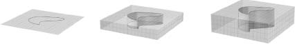
Figure 12.7 As the Heterotic-E string coupling constant is increased, a new space dimension appears and the string itself gets stretched into a cylindrical membrane shape.

This realization does not invalidate any of the conclusions we have drawn in previous chapters, but it does force us to see them within a new framework. For instance, how does this all mesh with the one time and nine space dimensions required by string theory? Well, recall from Chapter 8 that this constraint arises from counting the number of independent directions in which a string can vibrate, and requiring that this number be just right to ensure that quantum-mechanical probabilities have sensible values. The new dimension we have just uncovered is not one in which a Heterotic-E string can vibrate, since it is a dimension that is locked within the structure of the "strings" themselves. Put another way, the perturbative framework that physicists used in deriving the requirement of a ten-dimensional spacetime assumed from the outset that the Heterotic-E coupling constant is small. Although it was not recognized until much later, this implicitly enforced two mutually consistent approximations: that the width of the membrane in Figure 12.7 is small, making it look like a string, and that the eleventh dimension is so small that it is beyond the sensitivity of the perturbative equations. Within this approximation scheme, we are led to envision a ten-dimensional universe filled with one-dimensional strings. Now we see that this is but an approximation to an eleven-dimensional universe containing two-dimensional membranes.

For technical reasons, Witten first came upon the eleventh dimension in his studies of the strong coupling properties of the Type IIA string, and there the story is quite similar. As in the Heterotic-E example, there is an eleventh dimension whose size is controlled by the Type IIA coupling constant. When its value is increased, the new dimension grows. As it does, Witten argued, the Type IIA string, rather than stretching into a ribbon as in the Heterotic-E case, expands into an "inner tube," as illustrated in Figure 12.8. Once again, Witten argued that although theorists have always viewed Type IIA strings as one-dimensional objects, having only length but no thickness, this view is a reflection of the perturbative approximation scheme in which the string coupling constant is assumed to be small. If nature does require a small value of this coupling constant then it is a trustworthy approximation. Nevertheless, Witten's arguments and those of other physicists during the second superstring revolution do give strong evidence that the Type IIA and Heterotic-E "strings" are, fundamentally, two-dimensional membranes living in an eleven-dimensional universe.

But what is this eleven-dimensional theory? At low energies (low compared to the Planck energy), Witten and others argued, it is approximated by the long-neglected eleven-dimensional supergravity quantum field theory. But for higher energies, how can we describe this theory? This topic is currently under intense scrutiny. We know from Figures 12.7 and 12.8 that the eleven-dimensional theory contains two-dimensional extended objects—two-dimensional membranes. And as we shall soon discuss, extended objects of other dimensions play an important role as well. But beyond a hodgepodge of properties, no one knows what this eleven-dimensional theory is. Are membranes its fundamental ingredients? What are its defining properties? How does it purport to make contact with physics as we know it? If the respective coupling constants are small, our best current answers to these questions are described in previous chapters, since at small coupling constants we are led back to the theory of strings. But if the coupling constants are not small, no one currently knows the answers.

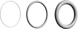
Figure 12.8 As the Type IIA string coupling constant is increased, strings expand from one-dimensional loops to two-dimensional objects that look like the surface of a bicycle-tire inner tube.

Whatever the eleven-dimensional theory is, Witten has provisionally named it M-theory. The name stands for as many things as people you poll. Some samples: Mystery Theory, Mother Theory (as in "Mother of all Theories"), Membrane Theory (since, whatever it is, membranes seem to be part of the story), Matrix Theory (after some recent work by Tom Banks of Rutgers University, Willy Fischler of the University of Texas at Austin, Stephen Shenker of Rutgers University, and Susskind that offers a novel interpretation of the theory). But even without having a firm grasp on its name or its properties, it is already clear that M-theory provides a unifying substrate for pulling together all five string theories.

M-Theory and the Web of Interconnections

There is an old proverb about three blind men and an elephant. The first blind man grabs hold of the elephant's ivory tusk and describes the smooth, hard surface that he feels. The second blind man grabs hold of one of the elephant's legs. He describes the tough, muscular girth that he feels. The third blind man grabs hold of the elephant's tail and describes the slender and sinewy appendage that he feels. Since their mutual descriptions are so different, and since none of the men can see the others, each thinks that he has grabbed hold of a different animal. For many years, physicists were as much in the dark as the blind men, thinking that the different string theories were very different. But now, through the insights of the second superstring revolution, physicists have realized that M-theory is the unifying pachyderm of the five string theories.

In this chapter we have discussed changes in our understanding of string theory that arise when we venture beyond the domain of the perturbative framework—a framework implicitly in use prior to this chapter. Figure 12.9 summarizes the interrelations we have found so far, with arrows to indicate dual theories. As you can see, we have a web of connections, but it is not yet complete. By also including the dualities of Chapter 10, we can finish the job.

Recall the large/small circular radius duality that interchanges a circular dimension of radius R with one whose radius is 1/R. Previously, we glossed over one aspect of this duality, which we now must clarify. In Chapter 10, we discussed the properties of strings in a universe with a circular dimension without carefully specifying which of the five string formulations we were working with. We argued that the interchange of winding and vibration modes of a string allows us to rephrase exactly the string theoretic description of a universe with a circular dimension of radius 1/R in terms of one in which the radius is R.The point we glossed over is that the Type IIA and Type IIB string theories actually get exchanged by this duality, as do the Heterotic-O and Heterotic-E strings. That is, the more precise statement of the large/small radius duality is this: The physics of the Type IIA string in a universe with a circular dimension of radius R is absolutely identical to the physics of the Type IIB string in a universe with a circular dimension of radius 1/R (a similar statement holds for the Heterotic-E and Heterotic-O strings). This refinement of the large/small radius duality has no significant effect on the conclusions of Chapter 10, but it does have an important impact on the present discussion.

Figure 12.9 The arrows show which theories are dual to others.

The reason is that by providing a link between the Type IIA and Type IIB string theories, as well as between the Heterotic-O and Heterotic-E theories, the large/small radius duality completes the web of connections, as illustrated by the dotted lines in Figure 12.10. This figure shows that all five string theories, together with M-theory, are dual to one another. They are all sewn together into a single theoretical framework; they provide five different approaches to describing one and the same underlying physics. For some or other application, one phrasing may be far more effective than another. For instance, it's far easier to work with the weakly coupled Heterotic-O theory than it is to work with the strongly coupled Type I string. Nevertheless, they describe exactly the same physics.

Figure 12.10 By including the dualities involving the geometrical form of spacetime (as in Chapter 10), all five of the string theories and M-Theory are joined together in a web of dualities.

The Overall Picture

We can now more fully understand the two figures—Figures 12.1 and 12.2—that we introduced in the beginning of this chapter to summarize the essential points. In Figure 12.1 we see that prior to 1995, without taking any dualities into account, we had five apparently distinct string theories. Various physicists worked on each, but without an understanding of the dualities they appeared to be different theories. Each of the theories had variable features such as the size of their coupling constant and the geometrical form and sizes of curled-up dimensions. The hope was (and still is) that these defining properties would be determined by the theory itself, but without the ability to determine them with the current approximate equations, physicists have naturally studied the physics that follows from a range of possibilities. This is represented in Figure 12.1 by the shaded regions—each point in such a region denotes one specific choice for the coupling constant and the curled-up geometry. Without invoking any dualities, we still have five disjointed (collections of) theories.

But now, if we apply all of the dualities we have discussed, then as we vary the coupling and geometric parameters, we can pass from any one theory to any other, so long as we also include the unifying central region of M-theory; this is shown in Figure 12.2. Even though we have only a scant understanding of M-theory, these indirect arguments lend strong support to the claim that it provides a unifying substrate for our five naively distinct string theories. Moreover, we have learned that M-theory is closely related to yet a sixth theory—eleven-dimensional supergravity—and this is recorded in Figure 12.11, a more precise version of Figure 12.2.¹³

Figure 12.11 illustrates that the fundamental ideas and equations of M-theory, although only partially understood at the moment, unify those of all of the formulations of string theory. M-theory is the theoretical elephant that has opened the eyes of string theorists to a far grander unifying framework.

Figure 12.11 By incorporating the dualities, all five string theories, eleven-dimensional supergravity, and M-theory are merged together into a unified framework.

A Surprising Feature of M-Theory: Democracy in Extension

When the string coupling constant is small in any of the upper five peninsular regions of the theory map in Figure 12.11, the fundamental ingredient of the theory appears to be a one-dimensional string. We have, however, just gained a new perspective on this observation. If we start in either the Heterotic-E or Type IIA regions and turn the value of the respective string coupling constants up, we migrate toward the center of the map in Figure 12.11, and what appeared to be one-dimensional strings stretch into two-dimensional membranes. Moreover, through a more or less intricate sequence of duality relations involving both the string coupling constants and the detailed form of the curled-up spatial dimensions, we can smoothly and continuously move from any point in Figure 12.11 to any other. Since the two-dimensional membranes we have come upon from the Heterotic-E and Type IIA perspectives can be followed as we migrate to any of the three other string formulations in Figure 12.11, we learn that each of the five string formulations involves two-dimensional membranes as well.

This raises two questions. First, are two-dimensional membranes the true fundamental ingredient of string theory? And second, having made the bold leap in the 1970s and early 1980s from zero-dimensional point particles to one-dimensional strings, and having now seen that string theory actually involves two-dimensional membranes, might it be that there are even higher-dimensional ingredients in the theory as well? As of this writing, the answers to these questions are not fully known, but the situation appears to be the following.

We relied heavily on supersymmetry to give us some understanding of each formulation of string theory beyond the domain of validity of perturbative approximation methods. In particular, the properties of BPS states, their masses and their force charges, are uniquely determined by supersymmetry, and this allowed us to understand some of their strongly coupled characteristics without having to perform direct calculations of unimaginable difficulty. In fact, through the initial efforts of Horowitz and Strominger, and through subsequent groundbreaking work of Polchinski, we now know even more about these BPS states. In particular, not only do we know their masses and the force charges they carry, but we also have a clear understanding of what they look like. And the picture is, perhaps, the most surprising development of all. Some of the BPS states are one-dimensional strings. Others are two-dimensional membranes. By now, these shapes are familiar. But, the surprise is that yet others are three-dimensional, four-dimensional—in fact, the range of possibilities encompasses every spatial dimension up to and including nine. String theory or M-theory, or whatever it is finally called, actually contains extended objects of a whole slew of different spatial dimensions. Physicists have coined the term three-brane to describe extended objects with three spatial dimensions, four-brane for those with four spatial dimensions, and so on up to nine-branes (and, more generally, for an object with p space dimensions, where p represents a whole number, physicists have coined the far from euphonious terminology p-brane). Sometimes, using this terminology, strings are described as one-branes, and membranes as two-branes. The fact that all of these extended objects are actually part of the theory has led Paul Townsend to declare a "democracy of branes."

Notwithstanding brane democracy, strings—one-dimensional extended objects—are special for the following reason. Physicists have shown that the mass of the extended objects of every dimension except for one-dimensional strings is inversely proportional to the value of the associated string coupling constant when we are in any of the five string regions of Figure 12.11. This means that with weak string coupling, in any of the five formulations, all but the strings will be enormously massive—orders of magnitude heavier than the Planck mass. Because they are so heavy and, therefore, from E = mc², require such unimaginably high energy to be produced, branes have only a small effect on much of physics (but not on all, as we shall see in the next chapter). However, when we venture outside the peninsular regions of Figure 12.11, the higher-dimensional branes become lighter and hence increasingly important.¹⁴

And so, the image you should have in mind is the following. In the central region of Figure 12.11, we have a theory whose fundamental ingredients are not just strings or membranes, but rather "branes" of a variety of dimensions, all more or less on equal footing. Currently, we do not have a firm grasp on many essential features of this full theory. But one thing we do know is that as we move from the central region to any of the peninsular regions, only the strings (or membranes curled up to look ever more like strings, as in Figures 12.7 and 12.8) are light enough to make contact with physics as we know it—the particles of Table 1.1 and the four forces through which they interact. The perturbative analyses string theorists have made use of for close to two decades have not been refined enough to discover even the existence of the super-massive extended objects of other dimensions; strings dominated the analyses and the theory was given the far-from-democratic name of string theory. Again, in these regions of Figure 12.11 we are justified, for most considerations, in ignoring all but the strings. In essence, this is what we have done so far in this book. We see now, though, that in actuality the theory is more rich than anyone previously imagined.

Does Any of This Solve the Unanswered Questions in String Theory?

Yes and no. We have managed to deepen our understanding by breaking free of certain conclusions that, in retrospect, were a consequence of perturbative approximate analyses rather than true string physics. But the current scope of our nonperturbative tools is quite limited. The discovery of the remarkable web of duality relations affords us far greater insight into string theory, but many issues remain unresolved. At present, for example, we do not know how to go beyond the approximate equations for the value of the string coupling constant—equations that, as we have seen, are too coarse to give us any useful information. Nor do we have any greater insight into why there are precisely three extended spatial dimensions, or how to choose the detailed form for the curled-up dimensions. These questions require more sharply honed nonperturbative methods than we currently possess.

What we do have is a far deeper understanding of the logical structure and theoretical reach of string theory. Prior to the realizations summarized in Figure 12.11, the strong coupling behavior of each string theory was a black box, a complete mystery. As on maps of old, the realm of strong coupling was uncharted territory, potentially filled with dragons and sea monsters. But now we see that although the journey to strong coupling may take us through unfamiliar regions of M-theory, it ultimately lands us back in the comfortable surrounds of weak coupling—albeit in the dual language of what was once thought to be a different string theory.

Duality and M-theory unite the five string theories and they suggest an important conclusion. It may well be that there aren't other surprises, on par with the ones just discussed, that are awaiting our discovery. Once a cartographer can fill in every region on a spherical globe of the earth, the map is done and geographical knowledge is complete. That's not to say explorations in Antarctica or on an isolated island in Micronesia are without scientific or cultural merit. It only means that the age of geographic discovery is over. The absence of blank spots on the globe ensures this. The "theory map" of Figure 12.11 plays a similar role for string theorists. It covers the entire range of theories that can be reached by setting sail from any one of the five string constructions. Although we are far from a full understanding of the terra incognita of M-theory, there are no blank regions on the map. Like the cartographer, the string theorist can now claim with guarded optimism that the spectrum of logically sound theories incorporating the essential discoveries of the past century—special and general relativity; quantum mechanics; gauge theories of the strong, weak, and electromagnetic forces; supersymmetry; extra dimensions of Kaluza and Klein—is fully mapped out by Figure 12.11.

The challenge to the string theorist—or perhaps we should say the M-theorist—is to show that some point on the theory map of Figure 12.11 actually describes our universe. To do this requires finding the full and exact equations whose solution will pick out this elusive point on the map, and then understanding the corresponding physics with sufficient precision to allow comparisons with experiment. As Witten has said, "Understanding what M-theory really is—the physics it embodies—would transform our understanding of nature at least as radically as occurred in any of the major scientific upheavals of the past."¹⁵This is the program for unification in the twenty-first century.