Complexity: A Guided Tour - Melanie Mitchell (2009)
Part I. Background and History
Chapter 4. Computation
Quo facto, quando orientur controversiae, non magis disputatione opus erit inter duos philosophos, quam inter duos Computistas. Sufficiet enim calamos in manus sumere sedereque ad abacos, et sibi mutuo dicere: Calculemus!
[If controversies were to arise, there would be no more need of disputation between two philosophers than between two accountants. For it would suffice to take their pencils in their hands, to sit down to their slates, and say to each other, “Let us calculate.”]
—G. Leibniz (Trans. B. Russell)
PEOPLE USUALLY THINK of computation as the thing that a computer does, such as calculations in spreadsheets, word processing, e-mail, and the like. And they usually think of a computer as the machine on one’s desk (or lap) that has electronic circuits inside, and usually a color monitor and a mouse, and that in the distant past used old-fashioned technology such as vacuum tubes. We also have a vague idea that our brains themselves are roughly like computers, with logic, memory, input, and output.
However, if you peruse some of the scholarly literature or seminar titles in complex systems, you will find the word computation used in some rather unfamiliar contexts: a biology book on “computation in cells and tissues”; a keynote lecture on “immune system computation”; an economics lecture concerning “the nature and limits of distributed computation in markets”; an article in a prestigious science journal on “emergent computation in plants.” And this is just a small sampling of such usage.
The notion of computation has come a long way since the early days of computers, and many scientists now view the phenomenon of computation as being widespread in nature. It is clear that cells, tissues, plants, immune systems, and financial markets do not work anything like the computer on your desk, so what exactly do these people mean by computation, and why do they call it that?
In order to set the stage for addressing this question in chapter 12, this chapter gives an overview of the history of ideas about computation and what can be computed, and describes basics of computational concepts used by scientists to understand natural complex systems.
What Is Computation and What Can Be Computed?
Information, as narrowly defined by Shannon, concerns the predictability of a message source. In the real world, however, information is something that is analyzed for meaning, that is remembered and combined with other information, and that produces results or actions. In short, information is processed via computation.
The meaning of computation has changed dramatically over the years. Before the late 1940s, computing meant performing mathematical calculations by hand (what nineteenth-century British schoolboys would have called “doing sums”). Computers were people who did such calculations. One of my former professors, Art Burks, used to tell us how he had married a “computer”—the term used for women who were enlisted during World War II to hand-calculate ballistic trajectories. Alice Burks was working as such a computer when she met Art.
Nowadays computation is what computers of the electronic variety do and what natural complex systems seem to do as well. But what exactly is computation, and how much can it accomplish? Can a computer compute anything, in principle, or does it have any limits? These are questions that were answered only in the mid-twentieth century.
Hilbert’s Problems and Gödel’s Theorem
The study of the foundations and limitations of computation, which led to the invention of electronic computers, was developed in response to a set of seemingly abstract (and abstruse) math problems. These problems were posed in the year 1900 at the International Congress of Mathematicians in Paris by the German mathematician David Hilbert.
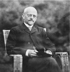
David Hilbert, 1862-1943 (AIP Emilio Segre Visual Archives, Lande Collection)
Hilbert’s lecture at this congress set out a list of mathematical New Year’s resolutions for the new century in the form of twenty-three of the most important unsolved problems in mathematics. Problems 2 and 10 ended up making the biggest splash. Actually, these were not just problems in mathematics; they were problems about mathematics itself and what can be proved by using mathematics. Taken together, these problems can be stated in three parts as follows:
1. Is mathematics complete? That is, can every mathematical statement be proved or disproved from a given finite set of axioms?
For example, remember Euclid’s axioms from high-school geometry? Remember using these axioms to prove statements such as “the angles in a triangle sum to 180 degrees”? Hilbert’s question was this: Given some fixed set of axioms, is there a proof for every true statement?
2. Is mathematics consistent? In other words, can only the true statements be proved? The notion of what is meant by “true statement” is technical, but I’ll leave it as intuitive. For example, if we could prove some false statement, such as 1 + 1 = 3, mathematics would be inconsistent and in big trouble.
3. Is every statement in mathematics decidable? That is, is there a definite procedure that can be applied to every statement that will tell us in finite time whether or not the statement is true or false? The idea here is that you could come up with a mathematical statement such as, “Every even integer greater than 2 can be expressed as the sum of two prime numbers,” hand it to a mathematician (or a computer), who would apply a precise recipe (a “definite procedure”), which would yield the correct answer “true” or “false” in finite time.
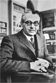
Kurt Gödel, 1906-1978 (Photograph courtesy of Princeton University Library)
The last question is known by its German name as the Entscheidungsproblem (“decision problem”), and goes back to the seventeenth-century mathematician Gottfried Leibniz. Leibniz actually built his own calculating machine, and believed that humans could eventually build a machine that could determine the truth or falsity of any mathematical statement.
Up until 1930, these three problems remained unsolved, but Hilbert expressed confidence that the answer would be “yes” in each case, and asserted that “there is no such thing as an unsolvable problem.”
However, his optimism turned out to be short-lived. Very short-lived. At the same meeting in 1930 at which Hilbert made his confident assertion, a twenty-five-year-old mathematician named Kurt Gödel astounded the mathematical world by presenting a proof of the so-called incompleteness theorem. This theorem stated that if the answer to question 2 above is “yes” (i.e., mathematics is consistent), then the answer to question 1 (is mathematics complete?) has to be “no.”
Gödel’s incompleteness theorem looked at arithmetic. He showed that if arithmetic is consistent, then there are true statements in arithmetic that cannot be proved—that is, arithmetic is incomplete. If arithmetic were inconsistent, then there would be false statements that could be proved, and all of mathematics would come crashing down.
Gödel’s proof is complicated. However, intuitively, it can be explained very easily. Gödel gave an example of a mathematical statement that can be translated into English as: “This statement is not provable.”
Think about it for a minute. It’s a strange statement, since it talks about itself—in fact, it asserts that it is not provable. Let’s call this statement “Statement A.” Now, suppose Statement A could indeed be proved. But then it would be false (since it states that it cannot be proved). That would mean a false statement could be proved—arithmetic would be inconsistent. Okay, let’s assume the opposite, that Statement A cannot be proved. That would mean that Statement A is true (because it asserts that it cannot be proved), but then there is a true statement that cannot be proved—arithmetic would be incomplete. Ergo, arithmetic is either inconsistent or incomplete.
It’s not easy to imagine how this statement gets translated into mathematics, but Gödel did it—therein lies the complexity and brilliance of Gödel’s proof, which I won’t cover here.
This was a big blow for the large number of mathematicians and philosophers who strongly believed that Hilbert’s questions would be answered affirmatively. As the mathematician and writer Andrew Hodges notes: “This was an amazing new turn in the enquiry, for Hilbert had thought of his programme as one of tidying up loose ends. It was upsetting for those who wanted to find in mathematics something that was perfect and unassailable….”
Turing Machines and Uncomputability
While Gödel dispatched the first and second of Hilbert’s questions, the British mathematician Alan Turing killed off the third.
In 1935 Alan Turing was a twenty-three-year-old graduate student at Cambridge studying under the logician Max Newman. Newman introduced Turing to Gödel’s recent incompleteness theorem. When he understood Gödel’s result, Turing was able to see how to answer Hilbert’s third question, the Entscheidungsproblem, and his answer, again, was “no.”
How did Turing show this? Remember that the Entscheidungsproblem asks if there is always a “definite procedure” for deciding whether a statement is provable. What does “definite procedure” mean? Turing’s first step was to define this notion. Following the intuition of Leibniz of more than two centuries earlier, Turing formulated his definition by thinking about a powerful calculating machine—one that could not only perform arithmetic but also could manipulate symbols in order to prove mathematical statements. By thinking about how humans might calculate, he constructed a mental design of such a machine, which is now called a Turing machine. The Turing machine turned out to be a blueprint for the invention of the electronic programmable computer.
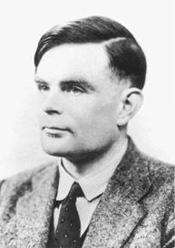
Alan Turing, 1912-1954 (Photograph copyright ©2003 by Photo Researchers Inc. Reproduced by permission.)
A QUICK INTRODUCTION TO TURING MACHINES
As illustrated in figure 4.1, a Turing machine consists of three parts: (1) A tape, divided into squares (or “cells”), on which symbols can be written and from which symbols can be read. The tape is infinitely long in both directions. (2) A movable read/write tape head that reads symbols from the tape and writes symbols to the tape. At any time, the head is in one of a number of states. (3) A set of rules that tell the head what to do next.
The head starts out at a particular tape cell and in a special start state. At each time step, the head reads the symbol at its current tape cell. The head then follows the rule that corresponds to that symbol and the head’s current state. The rule tells the head what symbol to write on the current tape cell (replacing the previous symbol); whether the head should move to the right, move to the left, or stay put; and what the head’s new state is. When the head goes into a special halt state, the machine is done and stops.
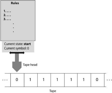
FIGURE 4.1. Illustration of a Turing machine.
The input to the machine is the set of symbols written on the tape before the machine starts. The output from the machine is the set of symbols written on the tape after the machine halts.
A SIMPLE EXAMPLE
A simple example will make all this clearer. To make things really simple, assume that (like a real computer) the only possible symbols that can be on a tape are 0, 1, and a blank symbol indicating a blank tape cell. Let’s design a Turing Machine that reads a tape containing all blank cells except for some number of 1s sandwiched between exactly two 0s (e.g., 011110) and determines whether the number of Is is even or odd. If even, then the final output of the machine will be a single 0 (and all other cells blank) on the tape. If odd, the final output will be a single 1 (and all other cells blank). Assume the input always has exactly two 0s on the tape, with zero or more 1s between them, and all blanks on either side of them.
Our Turing machine’s head will have four possible states: start, even, odd, and halt. The head will start on the left-most 0 and in the start state. We will write rules that cause the head to move to the right, one cell at a time, replacing the 0s and 1s it encounters with blanks. If the head reads a 1 in the current cell, the head goes into the odd state and moves one cell to the right. If it reads a 1 again it goes into the even state and moves one cell to the right, and so on, switching between the even and odd states as 1s are read.
When the head reads a 0, it has come to the end of the input, and whatever state it is in, odd or even, is the correct one. The machine will then write a corresponding 0 or 1 in its current cell and go into the halt state.
Here are the rules for the tape head that implement this algorithm:
1. If you are in the start state and read a 0, then change to the even state, replace the 0 with a blank (i.e., erase the 0), and move one cell to the right.
2. If you are in the even state and read a 1, change to the odd state, replace the 1 with a blank, and move one cell to the right.
3. If you are in the odd state and read a 1, change to the even state, replace the 1 with a blank, and move one cell to the right.
4. If you are in the odd state and read a 0, replace that 0 with a 1 and change to the halt state.
5. If you are in the even state and read a 0, replace that 0 with a 0 (i.e., don’t change it) and change to the halt state.
The process of starting with input symbols on the tape and letting the Turing machine serially process that input by using such rules is called “running the Turing machine on the input.”
Definite Procedures Defined as Turing Machines
In the example above, assuming that the input is in the correct format of zero or more 1s sandwiched between two 0s, running this Turing machine on the input is guaranteed to produce a correct answer for any input (including the special case of zero 1s, which is considered to be an even number). Even though it seems kind of clunky, you have to admit that this process is a “definite procedure”—a precise set of steps—for solving the even/odd problem. Turing’s first goal was to make very concrete this notion of definite procedure. The idea is that, given a particular problem to solve, you can construct a definite procedure for solving it by designing a Turing machine that solves it. Turing machines were put forth as the definition of “definite procedure,” hitherto a vague and ill-defined notion.
When formulating these ideas, Turing didn’t build any actual machines (though he built significant ones later on). Instead, all his thinking about Turing machines was done with pencil and paper alone.
Universal Turing Machines
Next, Turing proved an amazing fact about Turing machines: one can design a special universal Turing machine (let’s call it U) that can emulate the workings of any other Turing machine. For U to emulate a Turing machine Mrunning on an input I, U starts with part of its tape containing a sequence of 0s, 1s, and blanks that encodes input I, and part of its tape containing a sequence of 0s, 1s, and blanks that encodes machine M. The concept of encoding a machine M might not be familiar to you, but it is not hard. First, we recognize that all rules (like the five given in the “simple example” above) can be written in a shorthand that looks like
—Current State—Current Symbol—New State—New Symbol—Motion—
In this shorthand, Rule 1 above would be written as:
—start—0—even—blank—right—
(The separator ‘—’ is not actually needed, but makes the rule easier for us to read.) Now to encode a rule, we simply assign different three-digit binary numbers to each of the possible states: for example, start = 000, even = 001, odd = 010, and halt = 100. Similarly, we can assign three-digit binary numbers to each of the possible symbols: for example, symbol ‘0’ = 000, symbol ‘1’ = 001, and symbol blank = 100. Any such binary numbers will do, as long as each one represents only one symbol, and we are consistent in using them. It’s okay that the same binary number is used for, say, start and ‘0’; since we know the structure of the rule shorthand above, we will be able to tell what is being encoded from the context.
Similarly, we could encode “move right” by 000, and “move left” by 111. Finally, we could encode the ‘—’ separator symbol above as 111. Then we could, for example, encode Rule 1 as the string
111000111000111001111100111000111
which just substitutes our codes for the states and symbols in the shorthand above. The other rules would also be encoded in this way. Put the encoding strings all together, one after another, to form a single, long string, called the code of Turing machine M. To have U emulate M running on input I, U’s initial tape contains both input I and M’s code. At each step U reads the current symbol in I from the input part of the tape, decodes the appropriate rule from the M part of the tape, and carries it out on the input part, all the while keeping track (on some other part of its tape) of what state M would be in if M were actually running on the given input.
When M would have reached the halt state, U also halts, with the input (now output) part of its tape now containing the symbols M would have on its tape after it was run on the given input I. Thus we can say that “U runs M on I.” I am leaving out the actual states and rules of U, since they are pretty complicated, but I assure you that such a Turing machine can be designed. Moreover, what U does is precisely what a modern programmable computer does: it takes a program M that is stored in one part of memory, and runs it on an input I that is stored in another part of memory. It is notable that the first programmable computers were developed only ten years or so after Turing proved the existence of a universal Turing machine.
Turing’s Solution to the Entscheidungsproblem
Recall the question of the Entscheidungsproblem: Is there always a definite procedure that can decide whether or not a statement is true?
It was the existence of a universal Turing machine that enabled Turing to prove that the answer is “no.” He realized that the input I to a Turing machine M could be the code of another Turing machine. This is equivalent to the input of a computer program being the lines of another computer program. For example, you might write a program using a word processor such as Microsoft Word, save it to a file, and then run the “Word Count” program on the file. Here, your program is an input to another program (Word Count), and the output is the number of words in your program. The Word Count program doesn’t run your program; it simply counts the words in it as it would for any file of text.
Analogously, you could, without too much difficulty, design a Turing machine M that counted the 1s in its input, and then run M on the code for a second Turing machine M’. M would simply count the 1s in M’’s code. Of course, the Universal Turing Machine U could have the code for M in the “program” part of its tape, have the code for M’ in the “input” part of its tape, and run M on M’. Just to be perverse, we could put the code for M in both the “program” and “input” parts of U’s tape, and have M run on its own code! This would be like having the Word Count program run on its own lines of code, counting the number of words it contains itself. No problem!
All this may seem fairly pedestrian to your computer-sophisticated mind, but at the time Turing was developing his proof, his essential insight—that the very same string of 0s and 1s on a tape could be interpreted as either a program or as input to another program—was truly novel.
Now we’re ready to outline Turing’s proof.
Turing proved that the answer to the Entscheidungsproblem is “no” by using a mathematical technique called “proof by contradiction.” In this technique, you first assume that the answer is “yes” and use further reasoning to show that this assumption leads to a contradiction, and so cannot be the case.
Turing first assumed that the answer is “yes,” that is, there is always a definite procedure that can decide whether or not a given statement is true. Turing then proposed the following statement:
Turing Statement: Turing machine M, given input I, will reach the halt state after a finite number of time steps.
By the first assumption, there is some definite procedure that, given M and I as input, will decide whether or not this particular statement is true. Turing’s proof shows that this assumption leads to a contradiction.
It is important to note that there are some Turing machines that never reach the halt state. For instance, consider a Turing machine similar to the one in our example above but with only two rules:
1. If you are in the start state and read a 0 or a 1, change to the even state and move one cell to the right.
2. If you are in the even state and read a 0 or a 1, change to the start state and move one cell to the left.
This is a perfectly valid Turing machine, but it is one that will never halt. In modern language we would describe its action as an “infinite loop”—behavior that is usually the result of a programming bug. Infinite loops don’t have to be so obvious; in fact, there are many very subtle ways to create an infinite loop, whose presence is then very hard to detect.
Our assumption that there is a definite procedure that will decide the Turing Statement is equivalent to saying that we can design a Turing machine that is an infinite loop detector.
More specifically, our assumption says that we can design a Turing machine H that, given the code for any machine M and any input I on its tape, will, in finite time, answer “yes” if M would halt on input I, and “no” if M would go into an infinite loop and never halt.
The problem of designing H is called the “Halting problem.” Note that H itself must always halt with either a “yes” or “no” answer. So H can’t simply run M on I, since there would be some possibility that M (and thus H) would never halt. H has to do its job in some less straightforward way.
It’s not immediately clear how it would work, but nonetheless we have assumed that our desired H exists. Let’s denote H(M, I) as the action of running H on input M and I. The output is “yes” (e.g., a single 1 on the tape) if Mwould halt on I and “no” (e.g., a single 0 on the tape) if M would not halt on I.
Now, said Turing, we create a modified version of H, called H’, that takes as input the code for some Turing machine M, and calculates H(M, M). That is, H’ performs the same steps that H would to determine whether M would halt on its own code M. However, make H’ different from H in what it does after obtaining a “yes” or a “no”. H just halts, with the answer on its tape. H’ halts only if the answer is “No, M does not halt on code M.” If the answer is “Yes, M does halt on code M,” H’ goes into an infinite loop and never halts.
Whew, this might be getting a bit confusing. I hope you are following me so far. This is the point in every Theory of Computation course at which students either throw up their hands and say “I can’t get my mind around this stuff!” or clap their hands and say “I love this stuff!”
Needless to say, I was the second kind of student, even though I shared the confusion of the first kind of student. Maybe you are the same. So take a deep breath, and let’s go on.
Now for Turing’s big question:
What does H’ do when given as input the code for H’ , namely, its own code? Does it halt?
At this point, even the second kind of student starts to get a headache. This is really hard to get your head around. But let’s try anyway.
First, suppose that H’ does not halt on input H’. But then we have a problem. Recall that H’, given as input the code for some Turing machine M, goes into an infinite loop if and only if M does halt on M. So H’ not halting on input M implies that M does halt on input M. See what’s coming? H’ not halting on input H’ implies that H’ does halt on input H’. But H’ can’t both halt and not halt, so we have a contradiction.
Therefore, our supposition that H’ does not halt on H’ was wrong, so H’ must halt on input H’. But now we have the opposite problem. H’ only halts on its input M if M does not halt on M. So H’ only halts on H’ if H’ does not halt on H’. Another contradiction!
These contradictions show that H’ can neither halt on input H’ nor go into an infinite loop on input H’. An actual machine has to do one or the other, so H’ can’t exist. Since everything that H’ does is allowed for a Turing machine, except possibly running H, we have shown that H itself cannot exist.
Thus—and this is Turing’s big result—there can be no definite procedure for solving the Halting problem. The Halting problem is an example that proves that the answer to the Entscheidungsproblem is “no”; not every mathematical statement has a definite procedure that can decide its truth or falsity. With this, Turing put the final nail in the coffin for Hilbert’s questions.
Turing’s proof of the uncomputability of the Halting problem, sketched above, uses precisely the same core idea as Gödel’s incompleteness proof. Gödel figured out a way to encode mathematical statements so that they could talk about themselves. Turing figured out a way to encode mathematical statements as Turing machines and thus run on one another.
At this point, I should summarize Turing’s momentous accomplishments. First, he rigorously defined the notion of “definite procedure.” Second, his definition, in the form of Turing machines, laid the groundwork for the invention of electronic programmable computers. Third, he showed what few people ever expected: there are limits to what can be computed.
The Paths of Gödel and Turing
The nineteenth century was a time of belief in infinite possibility in mathematics and science. Hilbert and others believed they were on the verge of realizing Leibniz’s dream: discovering an automatic way to prove or disprove any statement, thus showing that there is nothing mathematics could not conquer. Similarly, as we saw in chapter 2, Laplace and others believed that, using Newton’s laws, scientists could in principle predict everything in the universe.
In contrast, the discoveries in mathematics and physics of the early to middle twentieth century showed that such infinite possibility did not in fact exist. Just as quantum mechanics and chaos together quashed the hope of perfect prediction, Gödel’s and Turing’s results quashed the hope of the unlimited power of mathematics and computing. However, as a direct consequence of his negative answer to the Entscheidungsproblem, Turing set the stage for the next great discovery, electronic programmable computers, which have since changed almost everything about the way science is done and the way our lives are lived.
After publishing their complementary proofs in the 1930s, Turing and Gödel took rather different paths, though, like everyone else at that time, their lives were deeply affected by the rise of Hitler and the Third Reich. Gödel, in spite of suffering from on-and-off mental health problems, continued his work on the foundations of mathematics in Vienna until 1940, when he moved to the United States to avoid serving in the German army. (According to his biographer Hao Wang, while preparing for American citizenship Gödel found a logical inconsistency in the U.S. Constitution, and his friend Albert Einstein had to talk him out of discussing it at length during his official citizenship interview.)
Gödel, like Einstein, was made a member of the prestigious Institute for Advanced Study in Princeton and continued to make important contributions to mathematical logic. However, in the 1960s and 1970s, his mental health deteriorated further. Toward the end of his life he became seriously paranoid and was convinced that he was being poisoned. As a result, he refused to eat and eventually starved to death.
Turing also visited the Institute for Advanced Study and was offered a membership but decided to return to England. During World War II, he became part of a top-secret effort by the British government to break the so-called Enigma cipher that was being used by the German navy to encrypt communications. Using his expertise in logic and statistics, as well as progress in electronic computing, he took the lead in developing code-breaking machines that were eventually able to decrypt almost all Enigma communications. This gave Britain a great advantage in its fight against Germany and arguably was a key factor in the eventual defeat of the Nazis.
After the war, Turing participated in the development of one of the first programmable electronic computers (stemming from the idea of his universal Turing machine), at Manchester University. His interests returned to questions about how the brain and body “compute,” and he studied neurology and physiology, did influential work on the theory of developmental biology, and wrote about the possibility of intelligent computers. However, his personal life presented a problem to the mores of the day: he did not attempt to hide his homosexuality. Homosexuality was illegal in 1950s Britain; Turing was arrested for actively pursuing relationships with men and was sentenced to drug “therapy” to treat his “condition.” He also lost his government security clearance. These events may have contributed to his probable suicide in 1954. Ironically, whereas Gödel starved himself to avoid being (as he believed) poisoned, Turing died from eating a poisoned (cyanide-laced) apple. He was only 41.