Complexity: A Guided Tour - Melanie Mitchell (2009)
Part I. Background and History
Chapter 2. Dynamics, Chaos, and Prediction
It makes me so happy. To be at the beginning again, knowing almost nothing…. The ordinary-sized stuff which is our lives, the things people write poetry about—clouds—daffodils—waterfalls…. these things are full of mystery, as mysterious to us as the heavens were to the Greeks…It’s the best possible time to be alive, when almost everything you thought you knew is wrong.
—Tom Stoppard, Arcadia
DYNAMICAL SYSTEMS THEORY (or dynamics) concerns the description and prediction of systems that exhibit complex changing behavior at the macroscopic level, emerging from the collective actions of many interacting components. The word dynamic means changing, and dynamical systems are systems that change over time in some way. Some examples of dynamical systems are
The solar system (the planets change position over time)
The heart of a living creature (it beats in a periodic fashion rather than standing still)
The brain of a living creature (neurons are continually firing, neurotransmitters are propelled from one neuron to another, synapse strengths are changing, and generally the whole system is in a continual state of flux)
The stock market
The world’s population
The global climate
Dynamical systems include these and most other systems that you probably can think of. Even rocks change over geological time. Dynamical systems theory describes in general terms the ways in which systems can change, what types of macroscopic behavior are possible, and what kinds of predictions about that behavior can be made.
Dynamical systems theory has recently been in vogue in popular science because of the fascinating results coming from one of its intellectual offspring, the study of chaos. However, it has a long history, starting, as many sciences did, with the Greek philosopher Aristotle.
Early Roots of Dynamical Systems Theory
Aristotle was the author of one of the earliest recorded theories of motion, one that was accepted widely for over 1,500 years. His theory rested on two main principles, both of which turned out to be wrong. First, he believed that motion on Earth differs from motion in the heavens. He asserted that on Earth objects move in straight lines and only when something forces them to; when no forces are applied, an object comes to its natural resting state. In the heavens, however, planets and other celestial objects move continuously in perfect circles centered about the Earth. Second, Aristotle believed that earthly objects move in different ways depending on what they are made of. For example, he believed that a rock will fall to Earth because it is mainly composed of the element earth, whereas smoke will rise because it is mostly composed of the element air. Likewise, heavier objects, presumably containing more earth, will fall faster than lighter objects.
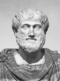
Aristotle, 384-322 B.C.
(Ludovisi Collection)
Clearly Aristotle (like many theorists since) was not one to let experimental results get in the way of his theorizing. His scientific method was to let logic and common sense direct theory; the importance of testing the resulting theories by experiments is a more modern notion. The influence of Aristotle’s ideas was strong and continued to hold sway over most of Western science until the sixteenth century—the time of Galileo.
Galileo was a pioneer of experimental, empirical science, along with his predecessor Copernicus and his contemporary Kepler. Copernicus established that the motion of the planets is centered not about the Earth but about the sun. (Galileo got into big trouble with the Catholic Church for promoting this view and was eventually forced to publicly renounce it; only in 1992 did the Church officially admit that Galileo had been unfairly persecuted.) In the early 1600s, Kepler discovered that the motion of the planets is not circular but rather elliptical, and he discovered laws describing this elliptical motion.
Whereas Copernicus and Kepler focused their research on celestial motion, Galileo studied motion not only in the heavens but also here on Earth by experimenting with the objects one now finds in elementary physics courses: pendula, balls rolling down inclined planes, falling objects, light reflected by mirrors. Galileo did not have the sophisticated experimental devices we have today: he is said to have timed the swinging of a pendulum by counting his heartbeats and to have measured the effects of gravity by dropping objects off the leaning tower of Pisa. These now-classic experiments revolutionized ideas about motion. In particular, Galileo’s studies directly contradicted Aristotle’s long-held principles of motion. Against common sense, rest is not the natural state of objects; rather it takes force to stop a moving object. Heavy and light objects in a vacuum fall at the same rate. And perhaps most revolutionary of all, laws of motion on the Earth could explain some aspects of motions in the heavens. With Galileo, the scientific revolution, with experimental observations at its core, was definitively launched.
The most important person in the history of dynamics was Isaac Newton. Newton, who was born the year after Galileo died, can be said to have invented, on his own, the science of dynamics. Along the way he also had to invent calculus, the branch of mathematics that describes motion and change.
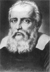
Galileo, 1564-1642 (AIP Emilio Segre Visual Archives, E. Scott Barr Collection)
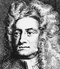
Isaac Newton, 1643-1727 (Original engraving by unknown artist, courtesy AIP Emilio Segre Visual Archives)
Physicists call the general study of motion mechanics. This is a historical term dating from ancient Greece, reflecting the classical view that all motion could be explained in terms of the combined actions of simple “machines” (e.g., lever, pulley, wheel and axle). Newton’s work is known today as classical mechanics. Mechanics is divided into two areas: kinematics, which describes how things move, and dynamics, which explains why things obey the laws of kinematics. For example, Kepler’s laws are kinematic laws—they describe how the planets move (in ellipses with the sun at one focus)—but not why they move in this particular way. Newton’s laws are the foundations of dynamics: they explain the motion of the planets, and everything else, in terms of the basic notions of force and mass.
Newton’s famous three laws are as follows:
1. Constant motion: Any object not subject to a force moves with unchanging speed.
2. Inertial mass: When an object is subject to a force, the resulting change in its motion is inversely proportional to its mass.
3. Equal and opposite forces: If object A exerts a force on object B, then object B must exert an equal and opposite force on object A.
One of Newton’s greatest accomplishments was to realize that these laws applied not just to earthly objects but to those in the heavens as well. Galileo was the first to state the constant-motion law, but he believed it applied only to objects on Earth. Newton, however, understood that this law should apply to the planets as well, and realized that elliptical orbits, which exhibit a constantly changing direction of motion, require explanation in terms of a force, namely gravity. Newton’s other major achievement was to state a universal law of gravity: the force of gravity between two objects is proportional to the product of their masses divided by the square of the distance between them. Newton’s insight—now the backbone of modern science—was that this law applies everywhere in the universe, to falling apples as well as to planets. As he wrote: “nature is exceedingly simple and conformable to herself. Whatever reasoning holds for greater motions, should hold for lesser ones as well.”
Newtonian mechanics produced a picture of a “clockwork universe,” one that is wound up with the three laws and then runs its mechanical course. The mathematician Pierre Simon Laplace saw the implication of this clockwork view for prediction: in 1814 he asserted that, given Newton’s laws and the current position and velocity of every particle in the universe, it was possible, in principle, to predict everything for all time. With the invention of electronic computers in the 1940s, the “in principle” might have seemed closer to “in practice.”
Revised Views of Prediction
However, two major discoveries of the twentieth century showed that Laplace’s dream of complete prediction is not possible, even in principle. One discovery was Werner Heisenberg’s 1927 “uncertainty principle” in quantum mechanics, which states that one cannot measure the exact values of the position and the momentum (mass times velocity) of a particle at the same time. The more certain one is about where a particle is located at a given time, the less one can know about its momentum, and vice versa. However, effects of Heisenberg’s principle exist only in the quantum world of tiny particles, and most people viewed it as an interesting curiosity, but not one that would have much implication for prediction at a larger scale—predicting the weather, say.
It was the understanding of chaos that eventually laid to rest the hope of perfect prediction of all complex systems, quantum or otherwise. The defining idea of chaos is that there are some systems—chaotic systems—in which even minuscule uncertainties in measurements of initial position and momentum can result in huge errors in long-term predictions of these quantities. This is known as “sensitive dependence on initial conditions.”
In parts of the natural world such small uncertainties will not matter. If your initial measurements are fairly but not perfectly precise, your predictions will likewise be close to right if not exactly on target. For example, astronomers can predict eclipses almost perfectly in spite of even relatively large uncertainties in measuring the positions of planets. But sensitive dependence on initial conditions says that in chaotic systems, even the tiniest errors in your initial measurements will eventually produce huge errors in your prediction of the future motion of an object. In such systems (and hurricanes may well be an example) any error, no matter how small, will make long-term predictions vastly inaccurate.
This kind of behavior is counterintuitive; in fact, for a long time many scientists denied it was possible. However, chaos in this sense has been observed in cardiac disorders, turbulence in fluids, electronic circuits, dripping faucets, and many other seemingly unrelated phenomena. These days, the existence of chaotic systems is an accepted fact of science.
It is hard to pin down who first realized that such systems might exist. The possibility of sensitive dependence on initial conditions was proposed by a number of people long before quantum mechanics was invented. For example, the physicist James Clerk Maxwell hypothesized in 1873 that there are classes of phenomena affected by “influences whose physical magnitude is too small to be taken account of by a finite being, [but which] may produce results of the highest importance.”
Possibly the first clear example of a chaotic system was given in the late nineteenth century by the French mathematician Henri Poincaré. Poincaré was the founder of and probably the most influential contributor to the modern field of dynamical systems theory, which is a major outgrowth of Newton’s science of dynamics. Poincaré discovered sensitive dependence on initial conditions when attempting to solve a much simpler problem than predicting the motion of a hurricane. He more modestly tried to tackle the so-called three-body problem: to determine, using Newton’s laws, the long-term motions of three masses exerting gravitational forces on one another. Newton solved the two-body problem, but the three-body problem turned out to be much harder. Poincaré tackled it in 1887 as part of a mathematics contest held in honor of the king of Sweden. The contest offered a prize of 2,500 Swedish crowns for a solution to the “many body” problem: predicting the future positions of arbitrarily many masses attracting one another under Newton’s laws. This problem was inspired by the question of whether or not the solar system is stable: will the planets remain in their current orbits, or will they wander from them? Poincaré started off by seeing whether he could solve it for merely three bodies.
He did not completely succeed—the problem was too hard. But his attempt was so impressive that he was awarded the prize anyway. Like Newton with calculus, Poincaré had to invent a new branch of mathematics, algebraic topology, to even tackle the problem. Topology is an extended form of geometry, and it was in looking at the geometric consequences of the three-body problem that he discovered the possibility of sensitive dependence on initial conditions. He summed up his discovery as follows:
If we knew exactly the laws of nature and the situation of the universe at the initial moment, we could predict exactly the situation of that same universe at a succeeding moment. But even if it were the case that the natural laws had no longer any secret for us, we could still only know the initial situation approximately. If that enabled us to predict the succeeding situation with the same approximation, that is all we require, and we should say that the phenomenon has been predicted, that it is governed by laws. But it is not always so; it may happen that small differences in the initial conditions produce very great ones in the final phenomenon. A small error in the former will produce an enormous error in the latter. Prediction becomes impossible….
In other words, even if we know the laws of motion perfectly, two different sets of initial conditions (here, initial positions, masses, and velocities for objects), even if they differ in a minuscule way, can sometimes produce greatly different results in the subsequent motion of the system. Poincaré found an example of this in the three-body problem.
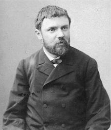
Henri Poincaré, 1854-1912 (AIP Emilio Segre Visual Archives)
It was not until the invention of the electronic computer that the scientific world began to see this phenomenon as significant. Poincaré, way ahead of his time, had guessed that sensitive dependence on initial conditions would stymie attempts at long-term weather prediction. His early hunch gained some evidence when, in 1963, the meteorologist Edward Lorenz found that even simple computer models of weather phenomena were subject to sensitive dependence on initial conditions. Even with today’s modern, highly complex meteorological computer models, weather predictions are at best reasonably accurate only to about one week in the future. It is not yet known whether this limit is due to fundamental chaos in the weather, or how much this limit can be extended by collecting more data and building even better models.
Linear versus Nonlinear Rabbits
Let’s now look more closely at sensitive dependence on initial conditions. How, precisely, does the huge magnification of initial uncertainties come about in chaotic systems? The key property is nonlinearity. A linear system is one you can understand by understanding its parts individually and then putting them together. When my two sons and I cook together, they like to take turns adding ingredients. Jake puts in two cups of flour. Then Nicky puts in a cup of sugar. The result? Three cups of flour/sugar mix. The whole is equal to the sum of the parts.
A nonlinear system is one in which the whole is different from the sum of the parts. Jake puts in two cups of baking soda. Nicky puts in a cup of vinegar. The whole thing explodes. (You can try this at home.) The result? Morethan three cups of vinegar-and-baking-soda-and-carbon-dioxide fizz.
The difference between the two examples is that in the first, the flour and sugar don’t really interact to create something new, whereas in the second, the vinegar and baking soda interact (rather violently) to create a lot of carbon dioxide.
Linearity is a reductionist’s dream, and nonlinearity can sometimes be a reductionist’s nightmare. Understanding the distinction between linearity and nonlinearity is very important and worthwhile. To get a better handle on this distinction, as well as on the phenomenon of chaos, let’s do a bit of very simple mathematical exploration, using a classic illustration of linear and nonlinear systems from the field of biological population dynamics.
Suppose you have a population of breeding rabbits in which every year all the rabbits pair up to mate, and each pair of rabbit parents has exactly four offspring and then dies. The population growth, starting from two rabbits, is illustrated in figure 2.1.
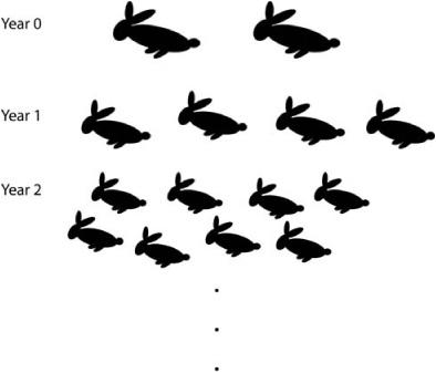
FIGURE 2.1. Rabbits with doubling population.
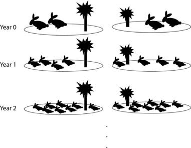
FIGURE 2.2. Rabbits with doubling population, split on two islands.
It is easy to see that the population doubles every year without limit (which means the rabbits would quickly take over the planet, solar system, and universe, but we won’t worry about that for now).
This is a linear system: the whole is equal to the sum of the parts. What do I mean by this? Let’s take a population of four rabbits and split them between two separate islands, two rabbits on each island. Then let the rabbits proceed with their reproduction. The population growth over two years is illustrated in figure 2.2.
Each of the two populations doubles each year. At each year, if you add the populations on the two islands together, you’ll get the same number of rabbits that you would have gotten had there been no separation—that is, had they all lived on one island.
If you make a plot with the current year’s population size on the horizontal axis and the next-year’s population size on the vertical axis, you get a straight line (figure 2.3). This is where the term linear system comes from.
But what happens when, more realistically, we consider limits to population growth? This requires us to make the growth rule nonlinear. Suppose that, as before, each year every pair of rabbits has four offspring and then dies. But now suppose that some of the offspring die before they reproduce because of overcrowding. Population biologists sometimes use an equation called the logistic model as a description of population growth in the presence of overcrowding. This sense of the word model means a mathematical formula that describes population growth in a simplified way.
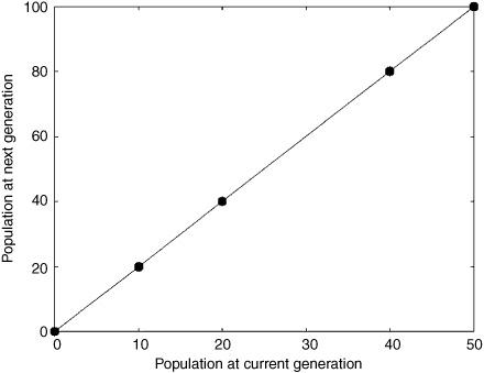
FIGURE 2.3. A plot of how the population size next year depends on the population size this year for the linear model.
In order to use the logistic model to calculate the size of the next generation’s population, you need to input to the logistic model the current generation’s population size, the birth rate, the death rate (the probability of an individual will die due to overcrowding), and the maximum carrying capacity (the strict upper limit of the population that the habitat will support.)
I won’t give the actual equation for the logistic model here (it is given in the notes), but you can see its behavior in figure 2.4.
As a simple example, let’s set birth rate = 2 and death rate = 0.4, assume the carrying capacity is thirty-two, and start with a population of twenty rabbits in the first generation. Using the logistic model, I calculate that the number of surviving offspring in the second generation is twelve. I then plug this new population size into the model, and find that there are still exactly twelve surviving rabbits in the third generation. The population will stay at twelve for all subsequent years.
If I reduce the death rate to 0.1 (keeping everything else the same), things get a little more interesting. From the model I calculate that the second generation has 14.25 rabbits and the third generation has 15.01816.
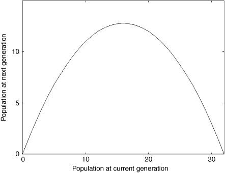
FIGURE 2.4. A plot of how the population size next year depends on the population size this year under the logistic model, with birth rate equal to 2, death rate equal to 0.4, and carrying capacity equal to 32. The plot will also be a parabola for other values of these parameters.
Wait a minute! How can we have 0.25 of a rabbit, much less 0.01816 of a rabbit? Obviously in real life we cannot, but this is a mathematical model, and it allows for fractional rabbits. This makes it easier to do the math, and can still give reasonable predictions of the actual rabbit population. So let’s not worry about that for now.
This process of calculating the size of the next population again and again, starting each time with the immediately previous population, is called “iterating the model.”
What happens if the death rate is set back to 0.4 and carrying capacity is doubled to sixty-four? The model tells me that, starting with twenty rabbits, by year nine the population reaches a value close to twenty-four and stays there.
You probably noticed from these examples that the behavior is more complicated than when we simply doubled the population each year. That’s because the logistic model is nonlinear, due to its inclusion of death by overcrowding. Its plot is a parabola instead of a line (figure 2.4). The logistic population growth is not simply equal to the sum of its parts. To show this, let’s see what happens if we take a population of twenty rabbits and segregate it into populations of ten rabbits each, and iterate the model for each population (with birth rate = 2 and death rate = .4, as in the first example above). The result is illustrated in figure 2.5.
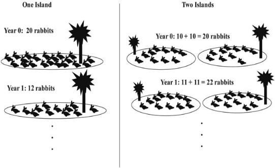
FIGURE 2.5. Rabbit population split on two islands, following the logistic model.
At year one, the original twenty-rabbit population has been cut down to twelve rabbits, but each of the original ten-rabbit populations now has eleven rabbits, for a total of twenty-two rabbits. The behavior of the whole is clearly not equal to the sum of the behavior of the parts.
The Logistic Map
Many scientists and mathematicians who study this sort of thing have used a simpler form of the logistic model called the logistic map, which is perhaps the most famous equation in the science of dynamical systems and chaos. The logistic model is simplified by combining the effects of birth rate and death rate into one number, called R. Population size is replaced by a related concept called “fraction of carrying capacity,” called x. Given this simplified model, scientists and mathematicians promptly forget all about population growth, carrying capacity, and anything else connected to the real world, and simply get lost in the astounding behavior of the equation itself. We will do the same.
Here is the equation, where xt is the current value of x and xt+1 is its value at the next time step:1
xt+1 = R xt (1 − xt).
I give the equation for the logistic map to show you how simple it is. In fact, it is one of the simplest systems to capture the essence of chaos: sensitive dependence on initial conditions. The logistic map was brought to the attention of population biologists in a 1971 article by the mathematical biologist Robert May in the prestigious journal Nature. It had been previously analyzed in detail by several mathematicians, including Stanislaw Ulam, John von Neumann, Nicholas Metropolis, Paul Stein, and Myron Stein. But it really achieved fame in the 1980s when the physicist Mitchell Feigenbaum used it to demonstrate universal properties common to a very large class of chaotic systems. Because of its apparent simplicity and rich history, it is a perfect vehicle to introduce some of the major concepts of dynamical systems theory and chaos.
The logistic map gets very interesting as we vary the value of R. Let’s start with R = 2. We need to also start out with some value between 0 and 1 for x0, say 0.5. If you plug those numbers into the logistic map, the answer for x1 is 0.5. Likewise, x2 = 0.5, and so on. Thus, if R = 2 and the population starts out at half the maximum size, it will stay there forever.
Now let’s try x0 = 0.2. You can use your calculator to compute this one. (I’m using one that reads off at most seven decimal places.) The results are more interesting:
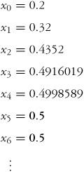
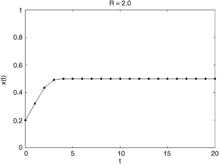
FIGURE 2.6. Behavior of the logistic map for R = 2 and x0 = 0.2.
The same eventual result (xt = 0.5 forever) occurs but here it takes five iterations to get there.
It helps to see these results visually. A plot of the value of xt at each time t for 20 time steps is shown in figure 2.6. I’ve connected the points by lines to better show how as time increases, x quickly converges to 0.5.
What happens if x0 is large, say, 0.99? Figure 2.7 shows a plot of the results.
Again the same ultimate result occurs, but with a longer and more dramatic path to get there.
You may have guessed it already: if R = 2 then xt eventually always gets to 0.5 and stays there. The value 0.5 is called a fixed point: how long it takes to get there depends on where you start, but once you are there, you are fixed.
If you like, you can do a similar set of calculations for R = 2.5, and you will find that the system also always goes to a fixed point, but this time the fixed point is 0.6.
For even more fun, let R = 3.1. The behavior of the logistic map now gets more complicated. Let x0 = 0.2. The plot is shown in figure 2.8.
In this case x never settles down to a fixed point; instead it eventually settles into an oscillation between two values, which happen to be 0.5580141 and 0.7645665. If the former is plugged into the formula the latter is produced, and vice versa, so this oscillation will continue forever. This oscillation will be reached eventually no matter what value is given for x0. This kind of regular final behavior (either fixed point or oscillation) is called an “attractor,” since, loosely speaking, any initial condition will eventually be “attracted to it.”
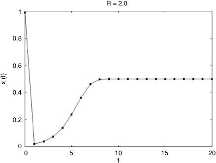
FIGURE 2.7. Behavior of the logistic map for R = 2 and x0 = 0.99.
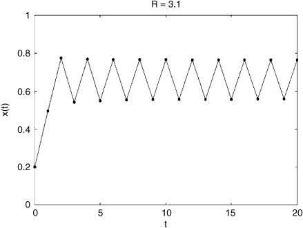
FIGURE 2.8. Behavior of the logistic map for R = 3.1 and x0 = 0.2.
For values of R up to around 3.4 the logistic map will have similar R.) Because it oscillates between two values, the system is said to have period equal to 2.
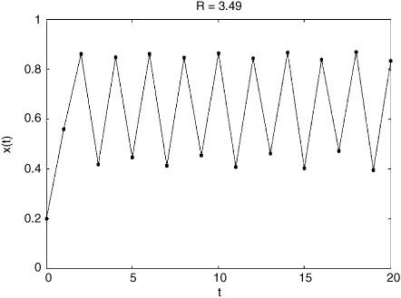
FIGURE 2.9. Behavior of the logistic map for R = 3.49 and x0 = 0.2.
But at a value between R = 3.4 and R = 3.5 an abrupt change occurs. Given any value of x0, the system will eventually reach an oscillation among four distinct values instead of two. For example, if we set R = 3.49, x0 = 0.2, we see the results in figure 2.9.
Indeed, the values of x fairly quickly reach an oscillation among four different values (which happen to be approximately 0.872, 0.389, 0.829, and 0.494, if you’re interested). That is, at some R between 3.4 and 3.5, the period of the final oscillation has abruptly doubled from 2 to 4.
Somewhere between R = 3.54 and R = 3.55 the period abruptly doubles again, jumping to 8. Somewhere between 3.564 and 3.565 the period jumps to 16. Somewhere between 3.5687 and 3.5688 the period jumps to 32. The period doubles again and again after smaller and smaller increases in R until, in short order, the period becomes effectively infinite, at an R value of approximately 3.569946. Before this point, the behavior of the logistic map was roughly predictable. If you gave me the value for R, I could tell you the ultimate long-term behavior from any starting point x0: fixed points are reached when R is less than about 3.1, period-two oscillations are reached when R is between 3.1 and 3.4, and so on.
When R is approximately 3.569946, the values of x no longer settle into an oscillation; rather, they become chaotic. Here’s what this means. Let’s call the series of values x0, x1, x2, and so on the trajectory of x. At values of R that yield chaos, two trajectories starting from very similar values of x0, rather than converging to the same fixed point or oscillation, will instead progressively diverge from each other. At R = 3.569946 this divergence occurs very slowly, but we can see a more dramatic sensitive dependence on x0 if we set R = 4.0. First I set x0 = 0.2 and iterate the logistic map to obtain a trajectory. Then I restarted with a new x0, increased slightly by putting a 1 in the tenth decimal place, x0 = 0.2000000001, and iterated the map again to obtain a second trajectory. In figure 2.10 the first trajectory is the dark curve with black circles, and the second trajectory is the light line with open circles.
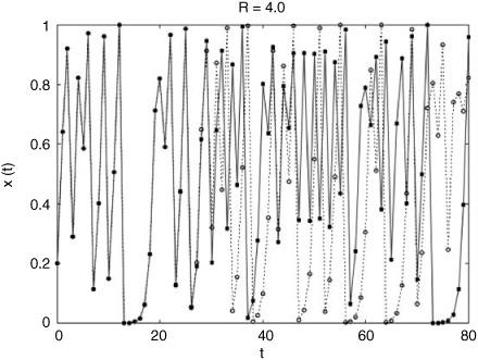
FIGURE 2.10. Two trajectories of the logistic map for R = 4.0: x0 = 0.2 and x0 = 0.2000000001.
The two trajectories start off very close to one another (so close that the first, solid-line trajectory blocks our view of the second, dashed-line trajectory), but after 30 or so iterations they start to diverge significantly, and soon after there is no correlation between them. This is what is meant by “sensitive dependence on initial conditions.”
So far we have seen three different classes of final behavior (attractors): fixed-point, periodic, and chaotic. (Chaotic attractors are also sometimes called “strange attractors.”) Type of attractor is one way in which dynamical systems theory characterizes the behavior of a system.
Let’s pause a minute to consider how remarkable the chaotic behavior really is. The logistic map is an extremely simple equation and is completely deterministic: every xt maps onto one and only one value of xt+1. And yet the chaotic trajectories obtained from this map, at certain values of R, look very random—enough so that the logistic map has been used as a basis for generating pseudo-random numbers on a computer. Thus apparent randomness can arise from very simple deterministic systems.
Moreover, for the values of R that produce chaos, if there is any uncertainty in the initial condition x0, there exists a time beyond which the future value cannot be predicted. This was demonstrated above with R = 4. If we don’t know the value of the tenth and higher decimal places of x0—a quite likely limitation for many experimental observations—then by t = 30 or so the value of xt is unpredictable. For any value of R that yields chaos, uncertainty in any decimal place of x0, however far out in the decimal expansion, will result in unpredictability at some value of t.
Robert May, the mathematical biologist, summed up these rather surprising properties, echoing Poincaré:
The fact that the simple and deterministic equation (1) [i.e., the logistic map] can possess dynamical trajectories which look like some sort of random noise has disturbing practical implications. It means, for example, that apparently erratic fluctuations in the census data for an animal population need not necessarily betoken either the vagaries of an unpredictable environment or sampling errors: they may simply derive from a rigidly deterministic population growth relationship such as equation (1)…. Alternatively, it may be observed that in the chaotic regime arbitrarily close initial conditions can lead to trajectories which, after a sufficiently long time, diverge widely. This means that, even if we have a simple model in which all the parameters are determined exactly, long-term prediction is nevertheless impossible.
In short, the presence of chaos in a system implies that perfect prediction à la Laplace is impossible not only in practice but also in principle, since we can never know x0 to infinitely many decimal places. This is a profound negative result that, along with quantum mechanics, helped wipe out the optimistic nineteenth-century view of a clockwork Newtonian universe that ticked along its predictable path.
But is there a more positive lesson to be learned from studies of the logistic map? Can it help the goal of dynamical systems theory, which attempts to discover general principles concerning systems that change over time? In fact, deeper studies of the logistic map and related maps have resulted in an equally surprising and profound positive result—the discovery of universal characteristics of chaotic systems.
Universals in Chaos
The term chaos, as used to describe dynamical systems with sensitive dependence on initial conditions, was first coined by physicists T. Y. Li and James Yorke. The term seems apt: the colloquial sense of the word “chaos” implies randomness and unpredictability, qualities we have seen in the chaotic version of logistic map. However, unlike colloquial chaos, there turns out to be substantial order in mathematical chaos in the form of so-called universalfeatures that are common to a wide range of chaotic systems.
THE FIRST UNIVERSAL FEATURE: THE PERIOD-DOUBLING
ROUTE TO CHAOS
In the mathematical explorations we performed above, we saw that as R was increased from 2.0 to 4.0, iterating the logistic map for a given value of R first yielded a fixed point, then a period-two oscillation, then period four, then eight, and so on, until chaos was reached. In dynamical systems theory, each of these abrupt period doublings is called a bifurcation. This succession of bifurcations culminating in chaos has been called the “period doubling route to chaos.”
These bifurcations are often summarized in a so-called bifurcation diagram that plots the attractor the system ends up in as a function of the value of a “control parameter” such as R. Figure 2.11 gives such a bifurcation diagram for the logistic map. The horizontal axis gives R. For each value of R, the final (attractor) values of x are plotted. For example, for R = 2.9, x reaches a fixed-point attractor of x = 0.655. At R = 3.0, x reaches a period-two attractor. This can be seen as the first branch point in the diagram, when the fixed-point attractors give way to the period-two attractors. For R somewhere between 3.4 and 3.5, the diagram shows a bifurcation to a period-four attractor, and so on, with further period doublings, until the onset of chaos at R approximately equal to 3.569946.
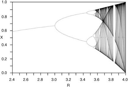
FIGURE 2.11. Bifurcation diagram for the logistic map, with attractor plotted as a function of R.
The period-doubling route to chaos has a rich history. Period doubling bifurcations had been observed in mathematical equations as early as the 1920s, and a similar cascade of bifurcations was described by P. J. Myrberg, a Finnish mathematician, in the 1950s. Nicholas Metropolis, Myron Stein, and Paul Stein, working at Los Alamos National Laboratory, showed that not just the logistic map but any map whose graph is parabola-shaped will follow a similar period-doubling route. Here, “parabola-shaped” means that plot of the map has just one hump—in mathematical terms, it is “unimodal.”
THE SECOND UNIVERSAL FEATURE: FEIGENBAUM’S
CONSTANT
The discovery that gave the period-doubling route its renowned place among mathematical universals was made in the 1970s by the physicist Mitchell Feigenbaum. Feigenbaum, using only a programmable desktop calculator, made a list of the R values at which the period-doubling bifurcations occur (where ≈ means “approximately equal to”):
R1 ≈ 3.0
R2 ≈ 3.44949
R3 ≈ 3.54409
R4 ≈ 3.564407
R5 ≈ 3.568759
R6 ≈ 3.569692
R7 ≈ 3.569891
R8 ≈ 3.569934
.
.
.
R∞ ≈ 3.569946
Here, R1 corresponds to period 21 (= 2), R2 corresponds to period 22 (= 4), and in general, Rn corresponds to period 2n. The symbol ∞ (“infinity”) is used to denote the onset of chaos—a trajectory with an infinite period.
Feigenbaum noticed that as the period increases, the R values get closer and closer together. This means that for each bifurcation, R has to be increased less than it had before to get to the next bifurcation. You can see this in the bifurcation diagram of Figure 2.11: as R increases, the bifurcations get closer and closer together. Using these numbers, Feigenbaum measured the rate at which the bifurcations get closer and closer; that is, the rate at which the Rvalues converge. He discovered that the rate is (approximately) the constant value 4.6692016. What this means is that as R increases, each new period doubling occurs about 4.6692016 times faster than the previous one.
This fact was interesting but not earth-shaking. Things started to get a lot more interesting when Feigenbaum looked at some other maps—the logistic map is just one of many that have been studied. As I mentioned above, a few years before Feigenbaum made these calculations, his colleagues at Los Alamos, Metropolis, Stein, and Stein, had shown that any unimodal map will follow a similar period-doubling cascade. Feigenbaum’s next step was to calculate the rate of convergence for some other unimodal maps. He started with the so-called sine map, an equation similar to the logistic map but which uses the trigonometric sine function.
Feigenbaum repeated the steps I sketched above: he calculated the values of R at the period-doubling bifurcations in the sine map, and then calculated the rate at which these values converged. He found that the rate of convergence was 4.6692016.
Feigenbaum was amazed. The rate was the same. He tried it for other unimodal maps. It was still the same. No one, including Feigenbaum, had expected this at all. But once the discovery had been made, Feigenbaum went on to develop a mathematical theory that explained why the common value of 4.6692016, now called Feigenbaum’s constant, is universal—which here means the same for all unimodal maps. The theory used a sophisticated mathematical technique called renormalization that had been developed originally in the area of quantum field theory and later imported to another field of physics: the study of phase transitions and other “critical phenomena.” Feigenbaum adapted it for dynamical systems theory, and it has become a cornerstone in the understanding of chaos.
It turned out that this is not just a mathematical curiosity. In the years since Feigenbaum’s discovery, his theory has been verified in several laboratory experiments on physical dynamical systems, including fluid flow, electronic circuits, lasers, and chemical reactions. Period-doubling cascades have been observed in these systems, and values of Feigenbaum’s constant have been calculated in steps similar to those we saw above. It is often quite difficult to get accurate measurements of, say, what corresponds to R values in such experiments, but even so, the values of Feigenbaum’s constant found by the experimenters agree well within the margin of error to Feigenbaum’s value of approximately 4.6692016. This is impressive, since Feigenbaum’s theory, which yields this number, involves only abstract math, no physics. As Feigenbaum’s colleague Leo Kadanoff said, this is “the best thing that can happen to a scientist, realizing that something that’s happened in his or her mind exactly corresponds to something that happens in nature.”

Mitchell Feigenbaum (AIP Emilio Segre Visual Archives, Physics Today Collection)
Large-scale systems such as the weather are, as yet, too hard to experiment with directly, so no one has directly observed period doubling or chaos in their behavior. However, certain computer models of weather have displayed the period-doubling route to chaos, as have computer models of electrical power systems, the heart, solar variability, and many other systems.
There is one more remarkable fact to mention about this story. Similar to many important scientific discoveries, Feigenbaum’s discoveries were also made, independently and at almost the same time, by another research team. This team consisted of the French scientists Pierre Coullet and Charles Tresser, who also used the technique of renormalization to study the period-doubling cascade and discovered the universality of 4.6692016 for unimodal maps. Feigenbaum may actually have been the first to make the discovery and was also able to more widely and clearly disseminate the result among the international scientific community, which is why he has received most of the credit for this work. However, in many technical papers, the theory is referred to as the “Feigenbaum-Coullet-Tresser theory” and Feigenbaum’s constant as the “Feigenbaum-Coullet-Tresser constant.” In the course of this book I point out several other examples of independent, simultaneous discoveries using ideas that are “in the air” at a given time.
Revolutionary Ideas from Chaos
The discovery and understanding of chaos, as illustrated in this chapter, has produced a rethinking of many core tenets of science. Here I summarize some of these new ideas, which few nineteenth-century scientists would have believed.
· Seemingly random behavior can emerge from deterministic systems, with no external source of randomness.
· The behavior of some simple, deterministic systems can be impossible, even in principle, to predict in the long term, due to sensitive dependence on initial conditions.
· Although the detailed behavior of a chaotic system cannot be predicted, there is some “order in chaos” seen in universal properties common to large sets of chaotic systems, such as the period-doubling route to chaos and Feigenbaum’s constant. Thus even though “prediction becomes impossible” at the detailed level, there are some higher-level aspects of chaotic systems that are indeed predictable.
In summary, changing, hard-to-predict macroscopic behavior is a hallmark of complex systems. Dynamical systems theory provides a mathematical vocabulary for characterizing such behavior in terms of bifurcations, attractors, and universal properties of the ways systems can change. This vocabulary is used extensively by complex systems researchers.
The logistic map is a simplified model of population growth, but the detailed study of it and similar model systems resulted in a major revamping of the scientific understanding of order, randomness, and predictability. This illustrates the power of idea models—models that are simple enough to study via mathematics or computers but that nonetheless capture fundamental properties of natural complex systems. Idea models play a central role in this book, as they do in the sciences of complex systems.
Characterizing the dynamics of a complex system is only one step in understanding it. We also need to understand how these dynamics are used in living systems to process information and adapt to changing environments. The next three chapters give some background on these subjects, and later in the book we see how ideas from dynamics are being combined with ideas from information theory, computation, and evolution.