Complexity: A Guided Tour - Melanie Mitchell (2009)
Part IV. Network Thinking
In Ersilia, to establish the relationships that sustain the city’s life, the inhabitants stretch strings from the corners of the houses, white or black or gray or black-and-white according to whether they mark a relationship of blood, of trade, authority, agency. When the strings become so numerous that you can no longer pass among them, the inhabitants leave: the houses are dismantled; only the strings and their supports remain.
From a mountainside, camping with their household goods, Ersilia’s refugees look at the labyrinth of taut strings and poles that rise in the plain. That is the city of Ersilia still, and they are nothing.
They rebuild Ersilia elsewhere. They weave a similar pattern of strings which they would like to be more complex and at the same time more regular than the other. Then they abandon it and take themselves and their houses still farther away.
Thus, when traveling in the territory of Ersilia, you come upon the ruins of abandoned cities, without the walls which do not last, without the bones of the dead which the wind rolls away: spiderwebs of intricate relationships seeking a form.
—Italo Calvino, Invisible Cities (Trans. W. Weaver)
Chapter 15. The Science of Networks
Small Worlds
I live in Portland, Oregon, whose metro area is home to over two million people. I teach at Portland State University, which has close to 25,000 students and over 1,200 faculty members. A few years back, my family had recently moved into a new house, somewhat far from campus, and I was chatting with our new next-door neighbor, Dorothy, a lawyer. I mentioned that I taught at Portland State. She said, “I wonder if you know my father. His name is George Lendaris.” I was amazed. George Lendaris is one of the three or four faculty members at PSU, including myself, who work on artificial intelligence. Just the day before, I had been in a meeting with him to discuss a grant proposal we were collaborating on. Small world!
Virtually all of us have had this kind of “small world” experience, many much more dramatic than mine. My husband’s best friend from high school turns out to be the first cousin of the guy who wrote the artificial intelligence textbook I use in my class. The woman who lived three houses away from mine in Santa Fe turned out to be a good friend of my high-school English teacher in Los Angeles. I’m sure you can think of several experiences of your own like this.
How is it that such unexpected connections seem to happen as often as they do? In the 1950s, a Harvard University psychologist named Stanley Milgram wanted to answer this question by determining, on average, how many links it would take to get from any person to any other person in the United States. He designed an experiment in which ordinary people would attempt to relay a letter to a distant stranger by giving the letter to an acquaintance, having the acquaintance give the letter to one of his or her acquaintances, and so on, until the intended recipient was reached at the end of the chain.
Milgram recruited (from newspaper ads) a group of “starters” in Kansas and Nebraska, and gave each the name, occupation, and home city of a “target,” a person unknown to the starter, to whom the letter was addressed. Two examples of Milgram’s chosen targets were a stockbroker in Boston and the wife of a divinity student in nearby Cambridge. The starters were instructed to pass on the letter to someone they knew personally, asking that person to continue the chain. Each link in the chain was recorded on the letter; if and when a letter reached the target, Milgram counted the number of links it went through. Milgram wrote of one example:
Four days after the folders were sent to a group of starting persons in Kansas, an instructor at the Episcopal Theological Seminary approached our target person on the street. “Alice,” he said, thrusting a brown folder toward her, “this is for you.” At first she thought he was simply returning a folder that had gone astray and had never gotten out of Cambridge, but when we looked at the roster, we found to our pleased surprise that the document had started with a wheat farmer in Kansas. He had passed it on to an Episcopalian minister in his home town, who sent it to the minister who taught in Cambridge, who gave it to the target person. Altogether, the number of intermediate links between starting person and target amounted to two!
In his most famous study, Milgram found that, for the letters that made it to their target, the median number of intermediate acquaintances from starter to target was five. This result was widely quoted and is the source of the popular notion that people are linked by only “six degrees of separation.”
Later work by psychologist Judith Kleinfeld has shown that the popular interpretation of Milgram’s work was rather skewed—in fact, most of the letters from starters never made it to their targets, and in other studies by Milgram, the median number of intermediates for letters that did reach the targets was higher than five. However, the idea of a small world linked by six degrees of separation has remained as what may be an urban myth of our culture. As Kleinfeld points out,
When people experience an unexpected social connection, the event is likely to be vivid and salient in a person’s memory .... We have a poor mathematical, as well as a poor intuitive understanding of the nature of coincidence.
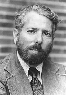
Stanley Milgram, 1933-1984. (Photograph by Eric Kroll, reprinted by permission of Mrs. Alexandra Milgram.)
So is it a small world or not? This question has recently received a lot of attention, not only for humans in the social realm, but also for other kinds of networks, ranging from the networks of metabolic and genetic regulation inside living cells to the explosively growing World Wide Web. Over the last decade questions about such networks have sparked a stampede of complex systems researchers to create what has been called the “new science of networks.”
The New Science of Networks
You’ve no doubt seen diagrams of networks like the one in figure 15.1. This one happens to be a map of the domestic flight routes of Continental Airlines. The dots (or nodes) represent cities and the lines (or links) represent flights between cities.
Airline route maps are an obvious example of the many natural, technological, and cultural phenomena that can usefully be described as networks. The brain is a huge network of neurons linked by synapses. The control of genetic activity in a cell is due to a complex network of genes linked by regulatory proteins. Social communities are networks in which the nodes are people (or organizations of people) between whom there are many different types of possible relationships. The Internet and the World Wide Web are of course two very prominent networks in today’s society. In the realm of national security, much effort has been put into identifying and analyzing possible “terrorist networks.”
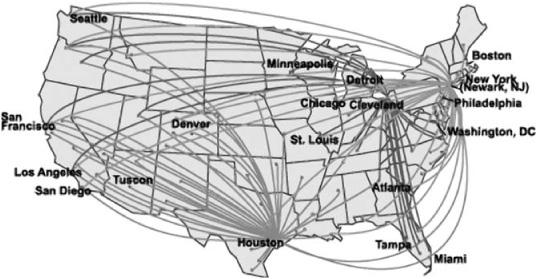
FIGURE 15.1. Slightly simplified route map of Continental Airlines. (From NASA Virtual Skies: [http://virtualskies.arc.nasa.gov/research/tutorial/tutorial2b.html].)
Until very recently, network science was not seen as a field unto itself. Mathematicians studied abstract network structures in a field called “graph theory.” Neuroscientists studied neural networks. Epidemiologists studied the transmission of diseases through networks of interacting people. Sociologists and social psychologists such as Milgram were interested in the structure of human social networks. Economists studied the behavior of economic networks, such as the spread of technological innovation in networks of businesses. Airline executives studied networks like the one in figure 15.1 in order to find a node-link structure that would optimize profits given certain constraints. These different groups worked pretty much independently, generally unaware of one another’s research.
However, over the last decade or so, a growing group of applied mathematicians and physicists have become interested in developing a set of unifying principles governing networks of any sort in nature, society, and technology. The seeds of this upsurge of interest in general networks were planted by the publication of two important papers in the late 1990s: “Collective Dynamics of ‘Small World Networks’ ” by Duncan Watts and Steven Strogatz, and “Emergence of Scaling in Random Networks” by Albert-László Barabási and Réka Albert. These papers were published in the world’s two top scientific journals, Nature and Science, respectively, and almost immediately got a lot of people really excited about this “new” field. Discoveries about networks started coming fast and furiously.
Duncan Watts (photograph courtesy of Duncan Watts).
The time and place was right for people to jump on this network-science rushing locomotive. A study of common properties of networks across disciplines is only feasible with computers fast enough to study networks empirically—both in simulation and with massive amounts of real-world data. By the 1990s, such work was possible. Moreover, the rising popularity of using the Internet for social, business, and scientific networking meant that large amounts of data were rapidly becoming available.
In addition, there was a large coterie of very smart physicists who had lost interest in the increasingly abstract nature of modern physics and were looking for something else to do. Networks, with their combination of pristine mathematical properties, complex dynamics, and real-world relevance, were the perfect vehicle. As Duncan Watts (who is an applied mathematician and sociologist) phrased it, “No one descends with such fury and in so great a number as a pack of hungry physicists, adrenalized by the scent of a new problem.” All these smart people were trained with just the right mathematical techniques, as well as the ability to simplify complex problems without losing their essential features. Several of these physicists-turned-network-scientists have become major players in this field.
Steven Strogatz (photograph courtesy of Steven Strogatz).

Albert-László Barabási (photograph courtesy of Albert-László Barabási).
Perhaps most important, there was, among many scientists, a progressive realization that new ideas, new approaches—really, a new way of thinking—were direly needed to help make sense of the highly complex, intricately connected systems that increasingly affect human life and well-being. Albert-László Barabási, among others, has labeled the resulting new approaches “network thinking,” and proclaimed that “network thinking is poised to invade all domains of human activity and most fields of human inquiry.”
What Is Network Thinking?
Network thinking means focusing on relationships between entities rather than the entities themselves. For example, as I described in chapter 7, the fact that humans and mustard plants each have only about 25,000 genes does not seem to jibe with the biological complexity of humans compared with these plants. In fact, in the last few decades, some biologists have proposed that the complexity of an organism largely arises from complexity in the interactionsamong its genes. I say much more about these interactions in chapter 18, but for now it suffices to say that recent results in network thinking are having significant impacts on biology.
Network thinking has recently helped to illuminate additional, seemingly unrelated, scientific and technological mysteries: Why is the typical life span of organisms a simple function of their size? Why do rumors, jokes, and “urban myths” spread so quickly? Why are large, complex networks such as electrical power grids and the Internet so robust in some circumstances, and so susceptible to large-scale failures in others? What types of events can cause a once-stable ecological community to fall apart?
Disparate as these questions are, network researchers believe that the answers reflect commonalities among networks in many different disciplines. The goals of network science are to tease out these commonalities and use them to characterize different networks in a common language. Network scientists also want to understand how networks in nature came to be and how they change over time.
The scientific understanding of networks could have a large impact not only on our understanding of many natural and social systems, but also on our ability to engineer and effectively use complex networks, ranging from better Web search and Internet routing to controlling the spread of diseases, the effectiveness of organized crime, and the ecological damage resulting from human actions.
What Is a ‘Network,’ Anyway?
In order to investigate networks scientifically, we have to define precisely what we mean by network. In simplest terms, a network is a collection of nodes connected by links. Nodes correspond to the individuals in a network (e.g., neurons, Web sites, people) and links to the connections between them (e.g., synapses, Web hyperlinks, social relationships).
For illustration, figure 15.2 shows part of my own social network—some of my close friends, some of their close friends, et cetera, with a total of 19 nodes. (Of course most “real” networks would be considerably larger.)
At first glance, this network looks like a tangled mess. However, if you look more closely, you will see some structure to this mess. There are some mutually connected clusters—not surprisingly, some of my friends are also friends with one another. For example, David, Greg, Doug, and Bob are all connected to one another, as are Steph, Ginger, and Doyne, with myself as a bridge between the two groups. Even knowing little about my history you might guess that these two “communities” of friends are associated with different interests of mine or with different periods in my life. (Both are true.)
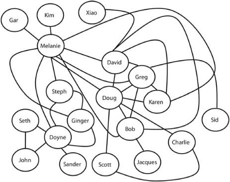
FIGURE 15.2. Part of my own social network.
You also might notice that there are some people with lots of friends (e.g., myself, Doyne, David, Doug, Greg) and some people with only one friend (e.g., Kim, Jacques, Xiao). Here this is due only to the incompleteness of this network, but in most large social networks there will always be some people with many friends and some people with few.
In their efforts to develop a common language, network scientists have coined terminology for these different kinds of network structures. The existence of largely separate tight-knit communities in networks is termed clustering. The number of links coming into (or out of) a node is called the degree of that node. For example, my degree is 10, and is the highest of all the nodes; Kim’s degree is 1 and is tied with five others for the lowest. Using this terminology, we can say that the network has a small number of high-degree nodes, and a larger number of low-degree ones.
This can be seen clearly in figure 15.3, where I plot the degree distribution of this network. For each degree from 1 to 10 the plot gives the number of nodes that have that degree. For example, there are six nodes with degree 1 (first bar) and one node with degree 10 (last bar).
This plot makes it explicit that there are many nodes with low degree and few nodes with high degree. In social networks, this corresponds to the fact that there are a lot of people with a relatively small number of friends, and a much smaller group of very popular people. Similarly, there are a small number of very popular Web sites (i.e., ones to which many other sites link), such as Google, with more than 75 million incoming links, and a much larger number of Web sites that hardly anyone has heard of—such as my own Web site, with 123 incoming links (many of which are probably from search engines).
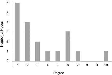
FIGURE 15.3. The degree distribution of the network in figure 15.2. For each degree, a bar is drawn representing the number of nodes with that degree.
High-degree nodes are called hubs; they are major conduits for the flow of activity or information in networks. Figure 15.1 illustrates the hub system that most airlines adopted in the 1980s, after deregulation: each airline designated certain cities as hubs, meaning that most of the airline’s flights go through those cities. If you’ve ever flown from the western United States to the East Coast on Continental Airlines, you probably had to change planes in Houston.
A major discovery to date of network science is that high-clustering, skewed degree distributions, and hub structure seem to be characteristic of the vast majority of all the natural, social, and technological networks that network scientists have studied. The presence of these structures is clearly no accident. If I put together a network by randomly sticking in links between nodes, all nodes would have similar degree, so the degree distribution wouldn’t be skewed the way it is in figure 15.3. Likewise, there would be no hubs and little clustering.
Why do networks in the real world have these characteristics? This is a major question of network science, and has been addressed largely by developing models of networks. Two classes of models that have been studied in depth are known as small-world networks and scale-free networks.
Small-World Networks
Although Milgram’s experiments may not have established that we actually live in a small world, the world of my social network (figure 15.2) is indeed small. That is, it doesn’t take many hops to get from any node to any other node. While they have never met one another (as far as I know), Gar can reach Charlie in only three hops, and John can reach Xiao in only four hops. In fact, in my network people are linked by at most four degrees of separation.
Applied mathematician and sociologist Duncan Watts and applied mathematician Steven Strogatz were the first people to mathematically define the concept of small-world network and to investigate what kinds of network structures have this property. (Their work on abstract networks resulted from an unlikely source: research on how crickets synchronize their chirps.) Watts and Strogatz started by looking at the simplest possible “regular” network: a ring of nodes, such as the network of figure 15.4, which has 60 nodes. Each node is linked to its two nearest neighbors in the ring, reminiscent of an elementary cellular automaton. To determine the degree of “small-worldness” in a network, Watts and Strogatz computed the average path length in the network. The path length between two nodes is simply the number of links on the shortest path between those two nodes. The average path length is simply the average over path lengths between all pairs of nodes in the network. The average path length of the regular network of figure 15.4 turns out to be 15. Thus, as in a children’s game of “telephone,” on average it would take a long time for a node to communicate with another node on the other side of the ring.
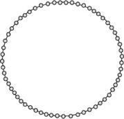
FIGURE 15.4. An example of a regular network. This network is a ring of nodes in which each node has a link to its two nearest neighbors.
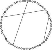
FIGURE 15.5. A random rewiring of three links turns the regular network of figure 15.4 into a small-world network.
Watts and Strogatz then asked, If we take a regular network like this and rewire it a little bit—that is, change a few of the nearest-neighbor links to long-distance links—how will this affect the average path length? They discovered that the effect is quite dramatic.
As an example, figure 15.5 shows the regular network of figure 15.4 with 5% (here, three) of the links rewired—that is, one end of each of the three links is moved to a randomly chosen node.
This rewired network has the same number of links as the original regular network, but the average path-length has shrunk to about 9. Watts and Strogatz found that as the number of nodes increases, the effect becomes increasingly pronounced. For example, in a regular network with 1,000 nodes, the average path length is 250; in the same network with 5% of the links randomly rewired, the average path length will typically fall to around 20. As Watts puts it, “only a few random links can generate a very large effect … on average, the first five random rewirings reduce the average path length of the network by one-half, regardless of the size of the network.”
These examples illustrate the small-world property: a network has this property if it has relatively few long-distance connections but has a small average path-length relative to the total number of nodes. Small-world networks also typically exhibit a high degree of clustering: for any nodes A, B, and C, if node A is connected to nodes B and C, then B and C are also likely to be connected to one another. This is not apparent in figure 15.5, since in this network most nodes are linked to only their two nearest neighbors. However, if the network were more realistic, that is, if each node were initially connected to multiple neighbors, the clustering would be high. An example is my own social network—I’m more likely to be friends with the friends of my friends than with other, random, people.
As part of their work, Watts and Strogatz looked at three examples of real-world networks from completely different domains and showed that they all have the small-world property. The first was a large network of movie actors. In this network, nodes represent individual actors; two nodes are linked if the corresponding actors have appeared in at least one movie together, such as Tom Cruise and Max von Sydow (Minority Report), or Cameron Diaz and Julia Roberts (My Best Friend’s Wedding). This particular social network has received attention via the popular “Kevin Bacon game,” in which a player tries to find the shortest path in the network from any given movie actor to the ultra-prolific actor Kevin Bacon. Evidently, if you are in movies and you don’t have a short path to Kevin Bacon, you aren’t doing so well in your career.
The second example is the electrical power grid of the western United States. Here, nodes represent the major entities in the power grid: electrical generators, transformers, and power substations. Links represent high-voltage transmission lines between these entities. The third example is the brain of the worm C. elegans, with nodes being neurons and links being connections between neurons. (Luckily for Watts and Strogatz, neuroscientists had already mapped out every neuron and neural connection in this humble worm’s small brain.)
You’d never have suspected that the “high-power” worlds of movie stars and electrical grids (not to mention the low-power world of a worm’s brain) would have anything interesting in common, but Watts and Strogatz showed that they are indeed all small-world networks, with low average path lengths and high clustering.
Watts and Strogatz’s now famous 1990 paper, “Collective Dynamics of ‘Small-World’ Networks,” helped ignite the spark that set the new science of networks aflame with activity. Scientists are finding more and more examples of small-world networks in the real world, some of which I’ll describe in the next chapter. Natural, social, and technological evolution seem to have produced organisms, communities, and artifacts with such structure. Why? It has been hypothesized that at least two conflicting evolutionary selective pressures are responsible: the need for information to travel quickly within the system, and the high cost of creating and maintaining reliable long-distance connections. Small-world networks solve both these problems by having short average path lengths between nodes in spite of having only a relatively small number of long-distance connections.
Further research showed that networks formed by the method proposed by Watts and Strogatz—starting with a regular network and randomly rewiring a small fraction of connections—do not actually have the kinds of degree distributions seen in many real-world networks. Soon, much attention was being paid to a different network model, one which produces scale-free networks—a particular kind of small-world network that looks more like networks in the real world.
Scale-Free Networks
I’m sure you have searched the World Wide Web, and you most likely use Google as your search engine. (If you’re reading this long after I wrote it in 2008, perhaps a new search engine has become predominant.) Back in the days of the Web before Google, search engines worked by simply looking up the words in your search query in an index that connected each possible English word to a list of Web pages that contained that word. For example, if your search query was the two words “apple records,” the search engine would give you a list of all the Web pages that included those words, in order of how many times those words appeared close together on the given page. You might be as likely to get a Web page about the historical price of apples in Washington State, or the fastest times recorded in the Great Apple Race in Tasmania, as you would a page about the famous record label formed in 1968 by the Beatles. It was very frustrating in those days to sort through a plethora of irrelevant pages to find the one with the information you were actually looking for.
In the 1990s Google changed all that with a revolutionary idea for presenting the results of a Web search, called “PageRank.” The idea was that the importance (and probable relevance) of a Web page is a function of how many other pages link to it (the number of “in-links”). For example, at the time I write this, the Web page with the American and Western Fruit Grower report about Washington State apple prices in 2008 has 39 in-links. The Web page with information about the Great Apple Race of Tasmania has 47 in-links. The Web page www.beatles.com has about 27,000 in-links. This page is among those presented at the top of the list for the “apple records” search. The other two are way down the list of approximately one million pages (“hits”) listed for this query. The original PageRank algorithm was a very simple idea, but it produced a tremendously improved search engine whereby the most relevant hits for a given query were usually at the top of the list.
If we look at the Web as a network, with nodes being Web pages and links being hyperlinks from one Web page to another, we can see that PageRank works only because this network has a particular structure: as in typical social networks, there are many pages with low degree (relatively few in-links), and a much smaller number of high-degree pages (i.e., relatively many in-links). Moreover, there is a wide variety in the number of in-links among pages, which allows ranking to mean something—to actually differentiate between pages. In other words, the Web has the skewed degree distribution and hub structure described above. It also turns out to have high clustering—different “communities” of Web pages have many mutual links to one another.
In network science terminology, the Web is a scale-free network. This has become one of the most talked-about notions in recent complex systems research, so let’s dig into it a bit, by looking more deeply at the Web’s degree distribution and what it means to be scale-free.
DEGREE DISTRIBUTION OF THE WEB
How can we figure out what the Web’s degree distribution is? There are two kinds of Web links: in-links and out-links. That is, suppose my page has a link to your page but not vice versa: I have an out-link and you have an in-link. One needs to be specific about which kinds of links are counted. The original PageRank algorithm looked only at in-links and ignored out-links—in this discussion I’ll do the same. We’ll call the number of in-links to a page the in-degree of that page.
Now, what is the Web’s in-degree distribution? It’s hard, if not impossible, to count all the pages and in-links on the Web—there’s no complete list stored anywhere and new links are constantly being added and old ones deleted. However, several Web scientists have tried to find approximate values using sampling and clever Web-crawling techniques. Estimates of the total number of Web pages vary considerably; as of 2008, the estimates I have seen range from 100 million to over 10 billion, and clearly the Web is still growing quickly.
Several different research groups have found that the Web’s in-degree distribution can be described by a very simple rule: the number of pages with a given in-degree is approximately proportional to 1 divided by the square of that in-degree. Suppose we denote the in-degree by the letter k. Then
Number of Web pages with in-degree k is proportional to ![]() .
.
(There has been some disagreement in the literature as to the actual exponent on k but it is close to 2—see the notes for details.) It turns out that this rule actually fits the data only for values of in-degree (k) in the thousands or greater.
To demonstrate why the Web is called “scale free,” I’ll plot the in-degree distribution as defined by this simple rule above, at three different scales. These plots are shown in figure 15.6. The first graph (top) plots the distribution for 9,000 in-degrees, starting at 1,000, which is close to where the rule becomes fairly accurate. Similar to figure 15.3, the in-degree values between 1,000 and 10,000 are shown on the horizontal axis, and their frequency (number of pages with the given in-degree) by the height of the boxes along the vertical axis. Here there are so many boxes that they form a solid black region.
The plots don’t give the actual values for frequency since I want to focus on the shape of the graph (not to mention that as far as I know, no one has very good estimates for the actual frequencies). However, you can see that there is a relatively large number of pages with k = 1,000 in-links, and this frequency quickly drops as in-degree increases. Somewhere between k = 5,000 and k = 10,000, the number of pages with k in-links is so small compared with the number of pages with 1,000 in-links that the corresponding boxes have essentially zero height.
What happens if we rescale—that is, zoom in on—this “near-zero-height” region? The second (middle) graph plots the in-degree distribution from k = 10,000 to k = 100,000. Here I’ve rescaled the plot so that the k = 10,000 box on this graph is at the same height as the k = 1,000 box on the previous graph. At this scale, there is now a relatively large number of pages with k = 10,000 in-links, and now somewhere between k = 50,000 and k = 100,000 we get “near-zero-height” boxes.
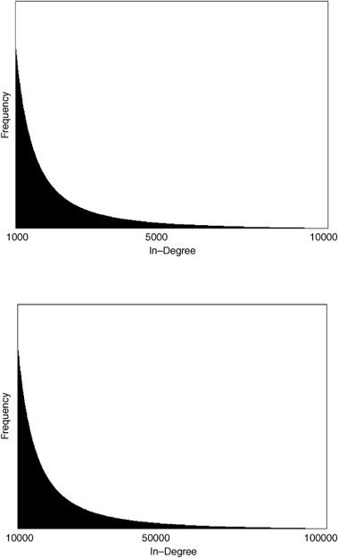
FIGURE 15.6. Approximate shape of the Web’s in-degree distribution at three different scales.
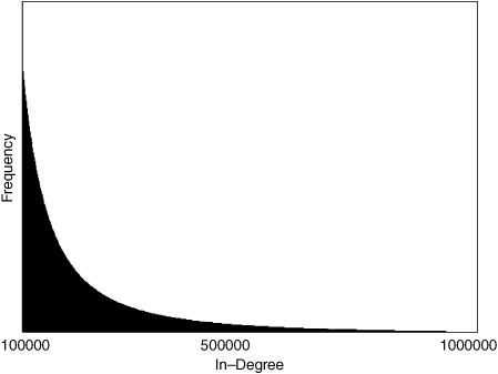
But something else is striking—except for the numbers on the horizontal axis, the second graph is identical to the first. This is true even though we are now plotting the distribution over 90,000 values instead of 9,000—what scientists call an order of magnitude more.
The third graph (bottom) shows the same phenomenon on an even larger scale. When we plot the distribution over k from 100,000 to 1 million, the shape remains identical.
A distribution like this is called self-similar, because it has the same shape at any scale you plot it. In more technical terms, it is “invariant under rescaling.” This is what is meant by the term scale-free. The term self-similaritymight be ringing a bell. We saw it back in chapter 7, in the discussion of fractals. There is indeed a connection to fractals here; more on this in chapter 17.
SCALE-FREE DISTRIBUTIONS VERSUS BELL CURVES
Scale-free networks are said to have no “characteristic scale.” This is best explained by comparing a scale-free distribution with another well-studied distribution, the so-called bell-curve.
Suppose I plotted the distribution of adult human heights in the world. The smallest (adult) person in the world is a little over 2 feet tall (around 70 cm). The tallest person is somewhere close to 9 feet tall (around 270 cm). The average adult height is about 5 feet 5 inches (165 cm), and the vast majority of all adults have height somewhere between 5 and 7 feet.
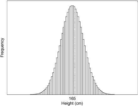
FIGURE 15.7. A bell-curve (normal) distribution of human heights.
The distribution of human heights looks something like figure 15.7. The plot’s bell-like shape is why it is often called a bell curve. Lots of things have approximate bell-curve distributions—height, weight, test scores on some exams, winning scores in basketball games, abundance of different species, and so on. In fact, because so many quantities in the natural world have this distribution, the bell curve is also called the normal distribution.
Normal distributions are characterized by having a particular scale—e.g., 70-270 cm for height, 0-100 for test scores. In a bell-curve distribution, the value with highest frequency is the average—e.g., 165 cm for height. Most other values don’t vary much from the average—the distribution is fairly homogeneous. If in-degrees in the Web were normally distributed, then PageRank wouldn’t work at all, since nearly all Web pages would have close to the average number of in-links. The Web page www.beatles.com would have more or less the same number of in-links as all other pages containing the phrase “apple records”; thus “number of in-links” could not be used as a way to rank such pages in order of probable relevance.
Fortunately for us (and even more so for Google stockholders), the Web degree distribution has a scale-free rather than bell-curve structure. Scale-free networks have four notable properties: (1) a relatively small number of very high-degree nodes (hubs); (2) nodes with degrees over a very large range of different values (i.e., heterogeneity of degree values); (3) self-similarity; (4) small-world structure. All scale-free networks have the small-world property, though not all networks with the small-world property are scale-free.
In more scientific terms, a scale-free network always has a power law degree distribution. Recall that the approximate in-degree distribution for the Web is
Number of Web pages with in-degree k is proportional to ![]() .
.
Perhaps you will remember from high school math that ![]() also can be written as k−2. This is a “power law with exponent −2.” Similarly,
also can be written as k−2. This is a “power law with exponent −2.” Similarly, ![]() (or, equivalently, k−1) is a power law with exponent −1.” In general, a power-law distribution has the form of xd, where x is a quantity such as in-degree. The key number describing the distribution is the exponent d; different exponents cause very different-looking distributions.
(or, equivalently, k−1) is a power law with exponent −1.” In general, a power-law distribution has the form of xd, where x is a quantity such as in-degree. The key number describing the distribution is the exponent d; different exponents cause very different-looking distributions.
I will have more to say about power laws in chapter 17. The important thing to remember for now is scale-free network = power-law degree distribution.
Network Resilience
A very important property of scale-free networks is their resilience to the deletion of nodes. This means that if a set of random nodes (along with their links) are deleted from a large scale-free network, the network’s basic properties do not change: it still will have a heterogeneous degree distribution, short average path length, and strong clustering. This is true even if the number of deleted nodes is fairly large. The reason for this is simple: if nodes are deleted at random, they are overwhelmingly likely to be low-degree nodes, since these constitute nearly all nodes in the network. Deleting such nodes will have little effect on the overall degree distribution and path lengths. We can see many examples of this in the Internet and the Web. Many individual computers on the Internet fail or are removed all the time, but this doesn’t have any obvious effect on the operation of the Internet or on its average path length. Similarly, although individual Web pages and their links are deleted all the time, Web surfing is largely unaffected.
However, this resilience comes at a price: if one or more of the hubs is deleted, the network will be likely to lose all its scale-free properties and cease to function properly. For example, a blizzard in Chicago (a big airline hub) will probably cause flight delays or cancellations all over the country. A failure in Google will wreak havoc throughout the Web.
In short, scale-free networks are resilient when it comes to random deletion of nodes but highly vulnerable if hubs go down or can be targeted for attack.
In the next chapter I discuss several examples of real-world networks that have been found to have small-world or scale-free properties and describe some theories of how they got that way.