Chaos: Making a New Science - James Gleick (1988)
Images of Chaos
What else, when chaos draws all forces inward To shape a single leaf.
—CONRAD AIKEN
MICHAEL BARNSLEY MET Mitchell Feigenbaum at a conference in Corsica in 1979. That was when Barnsley, an Oxford-educated mathematician, learned about universality and period-doubling and infinite cascades of bifurcations. A good idea, he thought, just the sort of idea that was sure to send scientists rushing to cut off pieces for themselves. For his part, Barnsley thought he saw a piece that no one else had noticed.
Where were these cycles of 2, 4, 8, 16, these Feigenbaum sequences, coming from? Did they appear by magic out of some mathematical void, or did they suggest the shadow of something deeper still. Barnsley’s intuition was that they must be part of some fabulous fractal object so far hidden from view.
For this idea, he had a context, the numerical territory known as the complex plane. In the complex plane, the numbers from minus infinity to infinity—all the real numbers, that is—lie on a line stretching from the far west to the far east, with zero at the center. But this line is only the equator of a world that also stretches to infinity in the north and the south. Each number is composed of two parts, a real part, corresponding to east-west longitude, and an imaginary part, corresponding to north-south latitude. By convention, these complex numbers are written this way: 2 + 3i, the i signifying the imaginary part. The two parts give each number a unique address in this two-dimensional plane. The original line of real numbers, then, is just a special case, the set of numbers whose imaginary part equals zero. In the complex plane, to look only at the real numbers—only at points on the equator—would be to limit one’s vision to occasional intersections of shapes that might reveal other secrets when viewed in two dimensions. So Barnsley suspected.
The names real and imaginary originated when ordinary numbers did seem more real than this new hybrid, but by now the names were recognized as quite arbitrary, both sorts of numbers being just as real and just as imaginary as any other sort. Historically, imaginary numbers were invented to fill the conceptual vacuum produced by the question: What is the square root of a negative number? By convention, the square root of -1 is i, the square root of -4 is 2i, and so on. It was only a short step to the realization that combinations of real and imaginary numbers allowed new kinds of calculations with polynomial equations. Complex numbers can be added, multiplied, averaged, factored, integrated. Just about any calculation on real numbers can be tried on complex numbers as well. Barnsley, when he began translating Feigenbaum functions into the complex plane, saw outlines emerging of a fantastical family of shapes, seemingly related to the dynamical ideas intriguing experimental physicists, but also startling as mathematical constructs.
These cycles do not appear out of thin air after all, he realized. They fall into the real line off the complex plane, where, if you look, there is a constellation of cycles, of all orders. There always was a two-cycle, a three-cycle, a four-cycle, floating just out of sight until they arrived on the real line. Barnsley hurried back from Corsica to his office at the Georgia Institute of Technology and produced a paper. He shipped it off to Communications in Mathematical Physics for publication. The editor, as it happened, was David Ruelle, and Ruelle had some bad news. Barnsley had unwittingly rediscovered a buried fifty-year-old piece of work by a French mathematician. “Ruelle shunted it back to me like a hot potato and said, ‘Michael, you’re talking about Julia sets,’” Barnsley recalled.
Ruelle added one piece of advice: “Get in touch with Mandelbrot.”
JOHN HUBBARD, AN AMERICAN MATHEMATICIAN with a taste for fashionable bold shirts, had been teaching elementary calculus to first-year university students in Orsay, France, three years before. Among the standard topics that he covered was Newton’s method, the classic scheme for solving equations by making successively better approximations. Hubbard was a little bored with standard topics, however, and for once he decided to teach Newton’s method in a way that would force his students to think.
Newton’s method is old, and it was already old when Newton invented it. The ancient Greeks used a version of it to find square roots. The method begins with a guess. The guess leads to a better guess, and the process of iteration zooms in on an answer like a dynamical system seeking its steady state. The process is fast, the number of accurate decimal digits generally doubling with each step. Nowadays, of course, square roots succumb to more analytic methods, as do all roots of degree-two polynomial equations—those in which variables are raised only to the second power. But Newton’s method works for higher-degree polynomial equations that cannot be solved directly. The method also works beautifully in a variety of computer algorithms, iteration being, as always, the computer’s forte. One tiny awkwardness about Newton’s method is that equations usually have more than one solution, particularly when complex solutions are included. Which solution the method finds depends on the initial guess. In practical terms, students find that this is no problem at all. You generally have a good idea of where to start, and if your guess seems to be converging to the wrong solution, you just start someplace else.
One might ask exactly what sort of route Newton’s method traces as it winds toward a root of a degree-two polynomial on the complex plane. One might answer, thinking geometrically, that the method simply seeks out whichever of the two roots is closer to the initial guess. That is what Hubbard told his students at Orsay when the question arose one day.
“Now, for equations of, say, degree three, the situation seems more complicated,” Hubbard said confidently. “I will think of it and tell you next week.”
He still presumed that the hard thing would be to teach his students how to calculate the iteration and that making the initial guess would be easy. But the more he thought about it, the less he knew—about what constituted an intelligent guess or, for that matter, about what Newton’s method really did. The obvious geometric guess would be to divide the plane into three equal pie wedges, with one root inside each wedge, but Hubbard discovered that that would not work. Strange things happened near the boundaries. Furthermore, Hubbard discovered that he was not the first mathematician to stumble on this surprisingly difficult question. Arthur Cayley had tried in 1879 to move from the manageable second-degree case to the frighteningly intractable third-degree case. But Hubbard, a century later, had a tool at hand that Cayley lacked.
Hubbard was the kind of rigorous mathematician who despised guesses, approximations, half-truths based on intuition rather than proof. He was the kind of mathematician who would continue to insist, twenty years after Edward Lorenz’s attractor entered the literature, that no one really knew whether those equations gave rise to a strange attractor. It was unproved conjecture. The familiar double spiral, he said, was not proof but mere evidence, something computers drew.
Now, in spite of himself, Hubbard began using a computer to do what the orthodox techniques had not done. The computer would prove nothing. But at least it might unveil the truth so that a mathematician could know what it was he should try to prove. So Hubbard began to experiment. He treated Newton’s method not as a way of solving problems but as a problem in itself. Hubbard considered the simplest example of a degree-three polynomial, the equation x3- 1 =0. That is, find the cube root of 1. In real numbers, of course, there is just the trivial solution: 1. But the polynomial also has two complex solutions: -½ + i√3/2, and -½ - i√3/2. Plotted in the complex plane, these three roots mark an equilateral triangle, with one point at three o’clock, one at seven o’clock, and one at eleven o’clock. Given any complex number as a starting point, the question was to see which of the three solutions Newton’s method would lead to. It was as if Newton’s method were a dynamical system and the three solutions were three attractors. Or it was as if the complex plane were a smooth surface sloping down toward three deep valleys. A marble starting from anywhere on the plane should roll into one of the valleys—but which?
Hubbard set about sampling the infinitude of points that make up the plane. He had his computer sweep from point to point, calculating the flow of Newton’s method for each one, and color-coding the results. Starting points that led to one solution were all colored blue. Points that led to the second solution were red, and points that led to the third were green. In the crudest approximation, he found, the dynamics of Newton’s method did indeed divide the plane into three pie wedges. Generally the points near a particular solution led quickly into that solution. But systematic computer exploration showed complicated underlying organization that could never have been seen by earlier mathematicians, able only to calculate a point here and a point there. While some starting guesses converged quickly to a root, others bounced around seemingly at random before finally converging to a solution. Sometimes it seemed that a point could fall into a cycle that would repeat itself forever—a periodic cycle—without ever reaching one of the three solutions.
As Hubbard pushed his computer to explore the space in finer and finer detail, he and his students were bewildered by the picture that began to emerge. Instead of a neat ridge between the blue and red valleys, for example, he saw blotches of green, strung together like jewels. It was as if a marble, caught between the conflicting tugs of two nearby valleys, would end up in the third and most distant valley instead. A boundary between two colors never quite forms. On even closer inspection, the line between a green blotch and the blue valley proved to have patches of red. And so on—the boundary finally revealed to Hubbard a peculiar property that would seem bewildering even to someone familiar with Mandelbrot’s monstrous fractals: no point serves as a boundary between just two colors. Wherever two colors try to come together, the third always inserts itself, with a series of new, self-similar intrusions. Impossibly, every boundary point borders a region of each of the three colors.
Hubbard embarked on a study of these complicated shapes and their implications for mathematics. His work and the work of his colleagues soon became a new line of attack on the problem of dynamical systems. He realized that the mapping of Newton’s method was just one of a whole unexplored family of pictures that reflected the behavior of forces in the real world. Michael Barnsley was looking at other members of the family. Benoit Mandelbrot, as both men soon learned, was discovering the granddaddy of all these shapes.
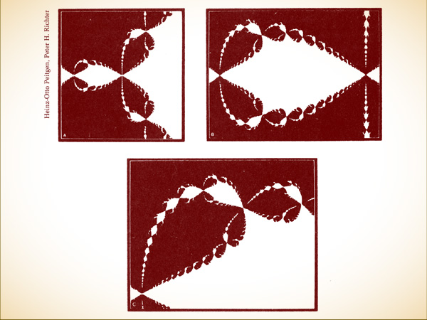
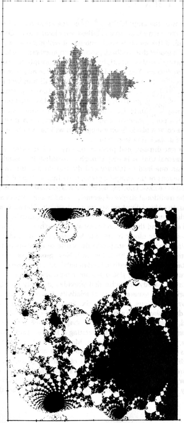
BOUNDARIES OF INFINITE COMPLEXITY. When a pie is cut into three slices, they meet at a single point, and the boundaries between any two slices are simple. But many processes of abstract mathematics and real-world physics turn out to create boundaries that are almost unimaginably complex.
Above, Newton’s method applied to finding the cube root of -1 divides the plane into three identical regions, one of which is shown in white. All white points are “attracted” to the root lying in the largest white area; all black points are attracted to one of the other two roots. The boundary has the peculiar property that every point on it borders all three regions. And, as the insets show, magnified segments reveal a fractal structure, repeating the basic pattern on smaller and smaller scales.
THE MANDELBROT SET IS the most complex object in mathematics, its admirers like to say. An eternity would not be enough time to see it all, its disks studded with prickly thorns, its spirals and filaments curling outward and around, bearing bulbous molecules that hang, infinitely variegated, like grapes on God’s personal vine. Examined in color through the adjustable window of a computer screen, the Mandelbrot set seems more fractal than fractals, so rich is its complication across scales. A cataloguing of the different images within it or a numerical description of the set’s outline would require an infinity of information. But here is a paradox: to send a full description of the set over a transmission line requires just a few dozen characters of code. A terse computer program contains enough information to reproduce the entire set. Those who were first to understand the way the set commingles complexity and simplicity were caught unprepared—even Mandelbrot. The Mandelbrot set became a kind of public emblem for chaos, appearing on the glossy covers of conference brochures and engineering quarterlies, forming the centerpiece of an exhibit of computer art that traveled internationally in 1985 and 1986. Its beauty was easy to feel from these pictures; harder to grasp was the meaning it had for the mathematicians who slowly understood it.
Many fractal shapes can be formed by iterated processes in the complex plane, but there is just one Mandelbrot set. It started appearing, vague and spectral, when Mandelbrot tried to find a way of generalizing about a class of shapes known as Julia sets. These were invented and studied during World War I by the French mathematicians Gaston Julia and Pierre Fatou, laboring without the pictures that a computer could provide. Mandelbrot had seen their modest drawings and read their work—already obscure—when he was twenty years old. Julia sets, in a variety of guises, were precisely the objects intriguing Barnsley. Some Julia sets are like circles that have been pinched and deformed in many places to give them a fractal structure. Others are broken into regions, and still others are disconnected dusts. But neither words nor the concepts of Euclidean geometry serve to describe them. The French mathematician Adrien Douady said: “You obtain an incredible variety of Julia sets: some are a fatty cloud, others are a skinny bush of brambles, some look like the sparks which float in the air after a firework has gone off. One has the shape of a rabbit, lots of them have sea-horse tails.”
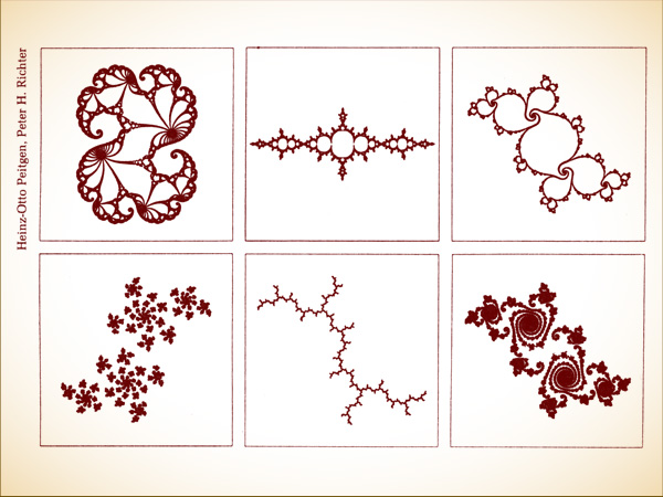
AN ASSORTMENT OF JULIA SETS.
In 1979 Mandelbrot discovered that he could create one image in the complex plane that would serve as a catalogue of Julia sets, a guide to each and every one. He was exploring the iteration of complicated processes, equations with square roots and sines and cosines. Even after building his intellectual life around the proposition that simplicity breeds complexity, he did not immediately understand how extraordinary was the object hovering just beyond the view of his computer screens at IBM and Harvard. He pressed his programmers hard for more detail, and they sweated over the allocation of already strained memory, the new interpolation of points on an IBM mainframe computer with a crude black and white display tube. To make matters worse, the programmers always had to stand guard against a common pitfall of computer exploration, the production of “artifacts,” features that sprang solely from some quirk of the machine and would disappear when a program was written differently.
Then Mandelbrot turned his attention to a simple mapping that was particularly easy to program. On a rough grid, with a program that repeated the feedback loop just a few times, the first outlines of disks appeared. A few lines of pencil calculation showed that the disks were mathematically real, not just products of some computational oddity. To the right and left of the main disks, hints of more shapes appeared. In his mind, he said later, he saw more: a hierarchy of shapes, atoms sprouting smaller atoms ad infinitum. And where the set intersected the real line, its successively smaller disks scaled with a geometric regularity that dynamicists now recognized: the Feigenbaum sequence of bifurcations.
That encouraged him to push the computation further, refining those first crude images, and he soon discovered dirt cluttering the edge of the disks and also floating in the space nearby. As he tried calculating in finer and finer detail, he suddenly felt that his string of good luck had broken. Instead of becoming sharper, the pictures became messier. He headed back to IBM’s Westchester County research center to try computing power on a proprietary scale that Harvard could not match. To his surprise, the growing messiness was the sign of something real. Sprouts and tendrils spun languidly away from the main island. Mandelbrot saw a seemingly smooth boundary resolve itself into a chain of spirals like the tails of sea horses. The irrational fertilized the rational.
The Mandelbrot set is a collection of points. Every point in the complex plane—that is, every complex number—is either in the set or outside it. One way to define the set is in terms of a test for every point, involving some simple iterated arithmetic. To test a point, take the complex number; square it; add the original number; square the result; add the original number; square the result—and so on, over and over again. If the total runs away to infinity, then the point is not in the Mandelbrot set. If the total remains finite (it could be trapped in some repeating loop, or it could wander chaotically), then the point is in the Mandelbrot set.
This business of repeating a process indefinitely and asking whether the result is infinite resembles feedback processes in the everyday world. Imagine that you are setting up a microphone, amplifier, and speakers in an auditorium. You are worried about the squeal of sonic feedback. If the microphone picks up a loud enough noise, the amplified sound from the speakers will feed back into the microphone in an endless, ever louder loop. On the other hand, if the sound is small enough, it will just die away to nothing. To model this feedback process with numbers, you might take a starting number, multiply it by itself, multiply the result by itself, and so on. You would discover that large numbers lead quickly to infinity: 10, 100, 10,000…. But small numbers lead to zero: ½, ¼ 1/16…. To make a geometric picture, you define a collection of all the points that, when fed into this equation, do not run away to infinity. Consider the points on a line from zero upward. If a point produces a squeal of feedback, color it white. Otherwise color it black. Soon enough, you will have a shape that consists of a black line from 0 to 1.
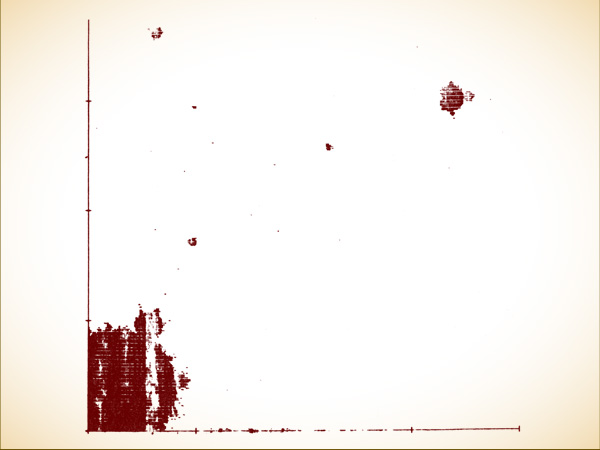
THE MANDELBROT SET EMERGES. In Benoit Mandelbrot’s first crude computer printouts, a rough structure appeared, gaining more detail as the quality of the computation improved. Were the buglike, floating “molecules” isolated islands? Or were they attached to the main body by filaments too fine to be observed? It was impossible to tell.
For a one-dimensional process, no one need actually resort to experimental trial. It is easy enough to establish that numbers greater than one lead to infinity and the rest do not. But in the two dimensions of the complex plane, to deduce a shape defined by an iterated process, knowing the equation is generally not enough. Unlike the traditional shapes of geometry, circles and ellipses and parabolas, the Mandelbrot set allows no shortcuts. The only way to see what kind of shape goes with a particular equation is by trial and error, and the trial-and-error style brought the explorers of this new terrain closer in spirit to Magellan than to Euclid.
Joining the world of shapes to the world of numbers in this way represented a break with the past. New geometries always begin when someone changes a fundamental rule. Suppose space can be curved instead of flat, a geometer says, and the result is a weird curved parody of Euclid that provides precisely the right framework for the general theory of relativity. Suppose space can have four dimensions, or five, or six. Suppose the number expressing dimension can be a fraction. Suppose shapes can be twisted, stretched, knotted. Or, now, suppose shapes are defined, not by solving an equation once, but by iterating it in a feedback loop.
Julia, Fatou, Hubbard, Barnsley, Mandelbrot—these mathematicians changed the rules about how to make geometrical shapes. The Euclidean and Cartesian methods of turning equations into curves are familiar to anyone who has studied high school geometry or found a point on a map using two coordinates. Standard geometry takes an equation and asks for the set of numbers that satisfy it. The solutions to an equation like x2 + y2 = 1, then, form a shape, in this case a circle. Other simple equations produce other pictures, the ellipses, parabolas, and hyperbolas of conic sections or even the more complicated shapes produced by differential equations in phase space. But when a geometer iterates an equation instead of solving it, the equation becomes a process instead of a description, dynamic instead of static. When a number goes into the equation, a new number comes out; the new number goes in, and so on, points hopping from place to place. A point is plotted not when it satisfies the equation but when it produces a certain kind of behavior. One behavior might be a steady state. Another might be a convergence to a periodic repetition of states. Another might be an out-of-control race to infinity.
Before computers, even Julia and Fatou, who understood the possibilities of this new kind of shape-making, lacked the means of making it a science. With computers, trial-and-error geometry became possible. Hubbard explored Newton’s method by calculating the behavior of point after point, and Mandelbrot first viewed his set the same way, using a computer to sweep through the points of the plane, one after another. Not all the points, of course. Time and computers being finite, such calculations use a grid of points. A finer grid gives a sharper picture, at the expense of longer computation. For the Mandelbrot set, the calculation was simple, because the process itself was so simple: the iteration in the complex plane of the mapping z→z2 + c. Take a number, multiply it by itself, and add the original number.
As Hubbard grew comfortable with this new style of exploring shapes by computer, he also brought to bear an innovative mathematical style, applying the methods of complex analysis, an area of mathematics that had not been applied to dynamical systems before. Everything was coming together, he felt. Separate disciplines within mathematics were converging at a crossroads. He knew it would not suffice to see the Mandelbrot set; before he was done, he wanted to understand it, and indeed, he finally claimed that he did understand it.
If the boundary were merely fractal in the sense of Mandelbrot’s turn-of-the-century monsters, then one picture would look more or less like the last. The principle of self-similarity at different scales would make it possible to predict what the electronic microscope would see at the next level of magnification. Instead, each foray deeper into the Mandelbrot set brought new surprises. Mandelbrot started worrying that he had offered too restrictive a definition of fractal; he certainly wanted the word to apply to this new object. The set did prove to contain, when magnified enough, rough copies of itself, tiny buglike objects floating off from the main body, but greater magnification showed that none of these molecules exactly matched any other. There were always new kinds of sea horses, new curling hothouse species. In fact, no part of the set exactly resembles any other part, at any magnification.
The discovery of floating molecules raised an immediate problem, though. Was the Mandelbrot set connected, one continent with far-flung peninsulas? Or was it a dust, a main body surrounded by fine islands? It was far from obvious. No guidance came from the experience with Julia sets, because Julia sets came in both flavors, some whole shapes and some dusts. The dusts, being fractal, have the peculiar property that no two pieces are “together”—because every piece is separated from every other by a region of empty space—yet no piece is “alone,” since whenever you find one piece, you can always find a group of pieces arbitrarily close by. As Mandelbrot looked at his pictures, he realized that computer experimentation was failing to settle this fundamental question. He focused more sharply on the specks hovering about the main body. Some disappeared, but others grew into clear near-replicas. They seemed independent. But possibly they were connected by lines so thin that they continued to escape the lattice of computed points.
Douady and Hubbard used a brilliant chain of new mathematics to prove that every floating molecule does indeed hang on a filigree that binds it to all the rest, a delicate web springing from tiny outcroppings on the main set, a “devil’s polymer,” in Mandelbrot’s phrase. The mathematicians proved that any segment—no matter where, and no matter how small—would, when blown up by the computer microscope, reveal new molecules, each resembling the main set and yet not quite the same. Every new molecule would be surrounded by its own spirals and flamelike projections, and those, inevitably, would reveal molecules tinier still, always similar, never identical, fulfilling some mandate of infinite variety, a miracle of miniaturization in which every new detail was sure to be a universe of its own, diverse and entire.
“EVERYTHING WAS VERY GEOMETRIC straight-line approaches,” said Heinz-Otto Peitgen. He was talking about modern art. “The work of Josef Albers, for example, trying to discover the relation of colors, this was essentially just squares of different colors put onto each other. These things were very popular. If you look at it now it seems to have passed. People don’t like it any more. In Germany they built huge apartment blocks in the Bauhaus style and people move out, they don’t like to live there. There are very deep reasons, it seems to me, in society right now to dislike some aspects of our conception of nature.” Peitgen had been helping a visitor select blowups of regions of the Mandelbrot set, Julia sets, and other complex iterative processes, all exquisitely colored. In his small California office he offered slides, large transparencies, even a Mandelbrot set calendar. “The deep enthusiasm we have has to do with this different perspective of looking at nature. What is the true aspect of the natural object? The tree, let’s say—what is important? Is it the straight line, or is it the fractal object?” At Cornell, meanwhile, John Hubbard was struggling with the demands of commerce. Hundreds of letters were flowing into the mathematics department to request Mandelbrot set pictures, and he realized he had to create samples and price lists. Dozens of images were already calculated and stored in his computers, ready for instant display, with the help of the graduate students who remembered the technical detail. But the most spectacular pictures, with the finest resolution and the most vivid coloration, were coming from two Germans, Peitgen and Peter H. Richter, and their team of scientists at the University of Bremen, with the enthusiastic sponsorship of a local bank.
Peitgen and Richter, one a mathematician and the other a physicist, turned their careers over to the Mandelbrot set. It held a universe of ideas for them: a modern philosophy of art, a justification of the new role of experimentation in mathematics, a way of bringing complex systems before a large public. They published glossy catalogs and books, and they traveled around the world with a gallery exhibit of their computer images. Richter had come to complex systems from physics by way of chemistry and then biochemistry, studying oscillations in biological pathways. In a series of papers on such phenomena as the immune system and the conversion of sugar into energy by yeast, he found that oscillations often governed the dynamics of processes that were customarily viewed as static, for the good reason that living systems cannot easily be opened up for examination in real time. Richter kept clamped to his windowsill a well-oiled double pendulum, his “pet dynamical system,” custom-made for him by his university machine shop. From time to time he would set it spinning in chaotic nonrhythms that he could emulate on a computer as well. The dependence on initial conditions was so sensitive that the gravitational pull of a single raindrop a mile away mixed up the motion within fifty or sixty revolutions, about two minutes. His multicolor graphic pictures of the phase space of this double pendulum showed the mingled regions of periodicity and chaos, and he used the same graphic techniques to display, for example, idealized regions of magnetization in a metal and also to explore the Mandelbrot set.
For his colleague Peitgen the study of complexity provided a chance to create new traditions in science instead of just solving problems. “In a brand new area like this one, you can start thinking today and if you are a good scientist you might be able to come up with interesting solutions in a few days or a week or a month,” Peitgen said. The subject is unstructured.
“In a structured subject, it is known what is known, what is unknown, what people have already tried and doesn’t lead anywhere. There you have to work on a problem which is known to be a problem, otherwise you get lost. But a problem which is known to be a problem must be hard, otherwise it would already have been solved.”
Peitgen shared little of the mathematicians’ unease with the use of computers to conduct experiments. Granted, every result must eventually be made rigorous by the standard methods of proof, or it would not be mathematics. To see an image on a graphics screen does not guarantee its existence in the language of theorem and proof. But the very availability of that image was enough to change the evolution of mathematics. Computer exploration was giving mathematicians the freedom to take a more natural path, Peitgen believed. Temporarily, for the moment, a mathematician could suspend the requirement of rigorous proof. He could go wherever experiments might lead him, just as a physicist could. The numerical power of computation and the visual cues to intuition would suggest promising avenues and spare the mathematician blind alleys. Then, new paths having been found and new objects isolated, a mathematician could return to standard proofs. “Rigor is the strength of mathematics,” Peitgen said. “That we can continue a line of thought which is absolutely guaranteed—mathematicians never want to give that up. But you can look at situations that can be understood partially now and with rigor perhaps in future generations. Rigor, yes, but not to the extent that I drop something just because I can’t do it now.”
By the 1980s a home computer could handle arithmetic precise enough to make colorful pictures of the set, and hobbyists quickly found that exploring these pictures at ever-greater magnification gave a vivid sense of expanding scale. If the set were thought of as a planet-sized object, a personal computer could show the whole object, or features the size of cities, or the size of buildings, or the size of rooms, or the size of books, or the size of letters, or the size of bacteria, or the size of atoms. The people who looked at such pictures saw that all the scales had similar patterns, yet every scale was different. And all these microscopic landscapes were generated by the same few lines of computer code.*
THE BOUNDARY IS WHERE a Mandelbrot set program spends most of its time and makes all of its compromises. There, when 100 or 1,000 or 10,000 iterations fail to break away, a program still cannot be absolutely certain that a point falls inside the step. Who knows what the millionth iteration will bring? So the programs that made the most striking, most deeply magnified pictures of the set ran on heavy mainframe computers, or computers devoted to parallel processing, with thousands of individual brains performing the same arithmetic in lock step. The boundary is where points are slowest to escape the pull of the set. It is as if they are balanced between competing attractors, one at zero and the other, in effect, ringing the set at a distance of infinity.
When scientists moved from the Mandelbrot set itself to new problems of representing real physical phenomena, the qualities of the set’s boundary came to the fore. The boundary between two or more attractors in a dynamical system served as a threshold of a kind that seems to govern so many ordinary processes, from the breaking of materials to the making of decisions. Each attractor in such a system has its basin, as a river has a watershed basin that drains into it. Each basin has a boundary. For an influential group in the early 1980s, a most promising new field of mathematics and physics was the study of fractal basin boundaries.
This branch of dynamics concerned itself not with describing the final, stable behavior of a system but with the way a system chooses between competing options. A system like Lorenz’s now-classic model has just one attractor in it, one behavior that prevails when the system settles down, and it is a chaotic attractor. Other systems may end up with nonchaotic steady-state behavior—but with more than one possible steady state. The study of fractal basin boundaries was the study of systems that could reach one of several nonchaotic final states, raising the question of how to predict which. James Yorke, who pioneered the investigation of fractal basin boundaries a decade after giving chaos its name, proposed an imaginary pinball machine. Like most pinball machines it has a plunger with a spring. You pull back the plunger and release it to send the ball up into the playing area. The machine has the customary tilted landscape of rubber edges and electric bouncers that give the ball a kick of extra energy. The kick is important: it means that energy does not just decay smoothly. For simplicity’s sake this machine has no flippers at the bottom, just two exit ramps. The ball must leave by one ramp or the other.
This is deterministic pinball—no shaking the machine. Only one parameter controls the ball’s destination, and that is the initial position of the plunger. Imagine that the machine is laid out so that a short pull of the plunger always means that the ball will end up rolling out the right-hand ramp, while a long pull always means that the ball will finish in the left-hand ramp. In between, the behavior gets complex, with the ball bouncing from bumper to bumper in the usual energetic, noisy, and variably long-lived manner before finally choosing one exit or the other.
Now imagine making a graph of the result of each possible starting position of the plunger. The graph is just a line. If a position leads to a right-hand departure, plot a red point, and plot a green point for left. What can we expect to find about these attractors as a function of the initial position?
The boundary proves to be a fractal set, not necessarily self-similar, but infinitely detailed. Some regions of the line will be pure red or green, while others, when magnified, will show new regions of red within the green, or green within the red. For some plunger positions, that is, a tiny change makes no difference. But for others, even an arbitrarily small change will make the difference between red and green.
To add a second dimension meant adding a second parameter, a second degree of freedom. With a pinball machine, for example, one might consider the effect of changing the tilt of the playing slope. One would discover a kind of in-and-out complexity that would give nightmares to engineers responsible for controlling the stability of sensitive, energetic real systems with more than one parameter—electrical power grids, for example, and nuclear generating plants, both of which became targets of chaos-inspired research in the 1980s. For one value of parameter A, parameter B might produce a reassuring, orderly kind of behavior, with coherent regions of stability. Engineers could make studies and graphs of exactly the kind their linear-oriented training suggested. Yet lurking nearby might be another value of parameter A that transforms the importance of parameter B.
Yorke would rise at conferences to display pictures of fractal basin boundaries. Some pictures represented the behavior of forced pendulums that could end up in one of two final states—the forced pendulum being, as his audiences well knew, a fundamental oscillator with many guises in everyday life. “Nobody can say that I’ve rigged the system by choosing a pendulum,” Yorke would say jovially. “This is the kind of thing you see throughout nature. But the behavior is different from anything you see in the literature. It’s fractal behavior of a wild kind.” The pictures would be fantastic swirls of white and black, as if a kitchen mixing bowl had sputtered a few times in the course of incompletely folding together vanilla and chocolate pudding. To make such pictures, his computer had swept through a 1,000 by 1,000 grid of points, each representing a different starting position for the pendulum, and had plotted the outcome: black or white. These were basins of attraction, mixed and folded by the familiar equations of Newtonian motion, and the result was more boundary than anything else. Typically, more than three-quarters of the plotted points lay on the boundary.
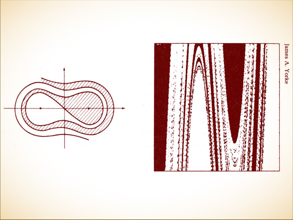
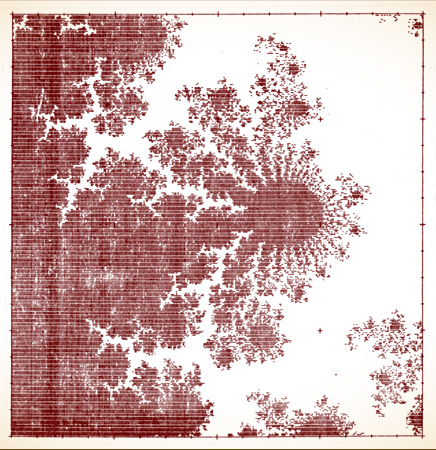
FRACTAL BASIN BOUNDARIES. Even when a dynamical system’s long-term behavior is not chaotic, chaos can appear at the boundary between one kind of steady behavior and another. Often a dynamical system has more than one equilibrium state, like a pendulum that can come to a halt at either of two magnets placed at its base. Each equilibrium is an attractor, and the boundary between two attractors can be complicated but smooth (left). Or the boundary can be complicated but not smooth. The highly fractal interspersing of white and black (right) is a phase-space diagram of a pendulum. The system is sure to reach one of two possible steady states. For some starting conditions, the outcome is quite predictable—black is black and white is white. But near the boundary, prediction becomes impossible.
To researchers and engineers, there was a lesson in these pictures—a lesson and a warning. Too often, the potential range of behavior of complex systems had to be guessed from a small set of data. When a system worked normally, staying within a narrow range of parameters, engineers made their observations and hoped that they could extrapolate more or less linearly to less usual behavior. But scientists studying fractal basin boundaries showed that the border between calm and catastrophe could be far more complex than anyone had dreamed. “The whole electrical power grid of the East Coast is an oscillatory system, most of the time stable, and you’d like to know what happens when you perturb it,” Yorke said. “You need to know what the boundary is. The fact is, they have no idea what the boundary looks like.”
Fractal basin boundaries addressed deep issues in theoretical physics. Phase transitions were matters of thresholds, and Peitgen and Richter looked at one of the best-studied kinds of phase transitions, magnetization and nonmagnetization in materials. Their pictures of such boundaries displayed the peculiarly beautiful complexity that was coming to seem so natural, cauliflower shapes with progressively more tangled knobs and furrows. As they varied the parameters and increased their magnification of details, one picture seemed more and more random, until suddenly, unexpectedly, deep in the heart of a bewildering region, appeared a familiar oblate form, studded with buds: the Mandelbrot set, every tendril and every atom in place. It was another signpost of universality. “Perhaps we should believe in magic,” they wrote.
MICHAEL BARNSLEY TOOK a different road. He thought about nature’s own images, particularly the patterns generated by living organisms. He experimented with Julia sets and tried other processes, always looking for ways of generating even greater variability. Finally, he turned to randomness as the basis for a new technique of modeling natural shapes. When he wrote about his technique, he called it “the global construction of fractals by means of iterated function systems.” When he talked about it, however, he called it “the chaos game.”
To play the chaos game quickly, you need a computer with a graphics screen and a random number generator, but in principle a sheet of paper and a coin work just as well. You choose a starting point somewhere on the paper. It does not matter where. You invent two rules, a heads rule and a tails rule. A rule tells you how to take one point to another: “Move two inches to the northeast,” or “Move 25 percent closer to the center.” Now you start flipping the coin and marking points, using the heads rule when the coin comes up heads and the tails rule when it comes up tails. If you throw away the first fifty points, like a blackjack dealer burying the first few cards in a new deal, you will find the chaos game producing not a random field of dots but a shape, revealed with greater and greater sharpness as the game goes on.
Barnsley’s central insight was this: Julia sets and other fractal shapes, though properly viewed as the outcome of a deterministic process, had a second, equally valid existence as the limit of a random process. By analogy, he suggested, one could imagine a map of Great Britain drawn in chalk on the floor of a room. A surveyor with standard tools would find it complicated to measure the area of these awkward shapes, with fractal coastlines, after all. But suppose you throw grains of rice into the air one by one, allowing them to fall randomly to the floor and counting the grains that land inside the map. As time goes on, the result begins to approach the area of the shapes—as the limit of a random process. In dynamical terms, Barnsley’s shapes proved to be attractors.
The chaos game made use of a fractal quality of certain pictures, the quality of being built up of small copies of the main picture. The act of writing down a set of rules to be iterated randomly captured certain global information about a shape, and the iteration of the rules regurgitated the information without regard to scale. The more fractal a shape was, in this sense, the simpler would be the appropriate rules. Barnsley quickly found that he could generate all the now-classic fractals from Mandelbrot’s book. Mandelbrot’s technique had been an infinite succession of construction and refinement. For the Koch snowflake or the Sierpiński gasket, one would remove line segments and replace them with specified figures. By using the chaos game instead, Barnsley made pictures that began as fuzzy parodies and grew progressively sharper. No refinement process was necessary: just a single set of rules that somehow embodied the final shape.
Barnsley and his co-workers now embarked on an out-of-control program of producing pictures, cabbages and molds and mud. The key question was how to reverse the process: given a particular shape, how to choose a set of rules. The answer, which he called “collage theorem,” was so inanely simple to describe that listeners sometimes thought there must be some trick. You would begin with a drawing of the shape you wanted to reproduce. Barnsley chose a black spleenwort fern for one of his first experiments, having long been a fern buff. Then using a computer terminal and a mouse as pointing device, you would lay small copies over the original shape, letting them overlap sloppily if need be. A highly fractal shape could easily be tiled with copies of itself, a less fractal shape less easily, and at some level of approximation every shape could be tiled.
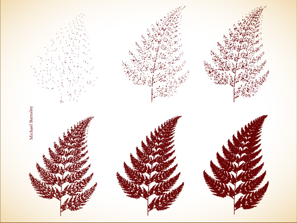
THE CHAOS GAME. Each new point falls randomly, but gradually the image of a fern emerges. All the necessary information is encoded in a few simple rules.
“If the image is complicated, the rules will be complicated,” Barnsley said. “On the other hand, if the object has a hidden fractal order to it—and it’s a central observation of Benoit’s that much of nature does have this hidden order—then it will be possible with a few rules to decode it. The model, then, is more interesting than a model made with Euclidean geometry, because we know that when you look at the edge of a leaf you don’t see straight lines.” His first fern, produced with a small desktop computer, perfectly matched the image in the fern book he had since he was a child. “It was a staggering image, correct in every aspect. No biologist would have any trouble identifying it.”
In some sense, Barnsley contended, nature must be playing its own version of the chaos game. “There’s only so much information in the spore that encodes one fern,” he said. “So there’s a limit to the elaborateness with which a fern could grow. It’s not surprising that we can find equivalent succinct information to describe ferns. It would be surprising if it were otherwise.”
But was chance necessary? Hubbard, too, thought about the parallels between the Mandelbrot set and the biological encoding of information, but he bristled at any suggestion that such processes might depend on probability. “There is no randomness in the Mandelbrot set,” Hubbard said. “There is no randomness in anything that I do. Neither do I think that the possibility of randomness has any direct relevance to biology. In biology randomness is death, chaos is death. Everything is highly structured. When you clone plants, the order in which the branches come out is exactly the same. The Mandelbrot set obeys an extraordinarily precise scheme leaving nothing to chance whatsoever. I strongly suspect that the day somebody actually figures out how the brain is organized they will discover to their amazement that there is a coding scheme for building the brain which is of extraordinary precision. The idea of randomness in biology is just reflex.”
In Barnsley’s technique, however, chance serves only as a tool. The results are deterministic and predictable. As points flash across the computer screen, no one can guess where the next one will appear; that depends on the flip of the machine’s internal coin. Yet somehow the flow of light always remains within the bounds necessary to carve a shape in phosphorous. To that extent the role of chance is an illusion. “Randomness is a red herring,” Barnsley said. “It’s central to obtaining images of a certain invariant measure that live upon the fractal object. But the object itself does not depend on the randomness. With probability one, you always draw the same picture.
“It’s giving deep information, probing fractal objects with a random algorithm. Just as, when we go into a new room, our eyes dance around it in some order which we might as well take to be random, and we get a good idea of the room. The room is just what it is. The object exists regardless of what I happen to do.”
The Mandelbrot set, in the same way, exists. It existed before Peitgen and Richter began turning it into an art form, before Hubbard and Douady understood its mathematical essence, even before Mandelbrot discovered it. It existed as soon as science created a context—a framework of complex numbers and a notion of iterated functions. Then it waited to be unveiled. Or perhaps it existed even earlier, as soon as nature began organizing itself by means of simple physical laws, repeated with infinite patience and everywhere the same.
______________
* A Mandelbrot set program needs just a few essential pieces. The main engine is a loop of instructions that takes its starting complex number and applies the arithmetical rule to it. For the Mandelbrot set, the rule is this: z→z2 + c, where z begins at zero and c is the complex number corresponding to the point being tested. So, take 0, multiply it by itself, and add the starting number; take the result—the starting number—multiply it by itself, and add the starting number; take the new result, multiply it by itself, and add the starting number. Arithmetic with complex numbers is straightforward. A complex number is written with two parts: for example, 2 + 3i (the address for the point at 2 east and 3 north on the complex plane). To add a pair of complex numbers, you just add the real parts to get a new real part and the imaginary parts to get a new imaginary part:
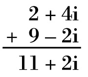
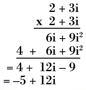
To multiply two complex numbers, you multiply each part of one number by each part of the other and add the four results together. Because i multiplied by itself equals -1, by the original definition of imaginary numbers, one term of the result collapses into another.
To break out of this loop, the program needs to watch the running total. If the total heads off to infinity, moving farther and farther from the center of the plane, the original point does not belong to the set, and if the running total becomes greater than 2 or smaller than - 2 in either its real or imaginary part, it is surely heading off to infinity—the program can move on. But if the program repeats the calculation many times without becoming greater than 2, then the point is part of the set. How many times depends on the amount of magnification. For the scales accessible to a personal computer, 100 or 200 is often plenty, and 1,000 is safe.
The program must repeat this process for each of thousands of points on a grid, with a scale that can be adjusted for greater magnification. And the program must display its result. Points in the set can be colored black, other points white. Or for a more vividly appealing picture, the white points can be replaced by colored gradations. If the iteration breaks off after ten repetitions, for example, a program might plot a red dot; for twenty repetitions an orange dot; for forty repetitions a yellow dot, and so on. The choice of colors and cutoff points can be adjusted to suit the programmer’s taste. The colors reveal the contours of the terrain just outside the set proper.