BioBuilder: Synthetic Biology in the Lab (2015)
Chapter 9. What a Colorful World
What a Colorful World emphasizes the “build” phase of the design-build-test cycle. The synthetic living systems you will build in this BioBuilder lab activity are cells colored with either a purple pigment or a green pigment, depending on the genetic program you choose to run. The intensity of the color, though, is tricky to predict in advance. Will the cells be pale or army green? Dark purple or light violet? Complicating things even further is the realization that each genetic circuit might produce different amounts of color depending on which bacterial strain is running it. The formal term for this kind of unexpected, quirky result from combining components is emergent behavior.
If you’re inclined to think like a scientist, such emergent behaviors might make you ask, “What explains the results I observe?” If you’re inclined to think like an engineer, these behaviors might make you think, “ugh”—and then get to work defining the best way to optimize a system’s performance with hopes of avoiding unexpected behaviors like these. Both approaches have merit, and together the scientific and engineering approaches should lead to more reliable designs in the future and minimize the number of surprising behaviors we see as we build new living systems.
In this lab, the DNA programs that generate purple or green pigments have already been written and assembled for you, but you will complete the final building step by inserting the DNA that encodes the programs into a few different bacterial chassis. The DNA programs come from a 2009 International Genetically Engineered Machines (iGEM) project called, “E. chromi,” in which students from the University of Cambridge designed and engineered E. coli to produce a spectrum of pigments. You will build several color-generating systems to explore how the chassis affects the output of a designed genetic program. Because the pigments are visible to the naked eye, you can easily decide whether the color outputs are different between chassis.
Before detailing the experiment, though, we will provide a general discussion of chassis design and decisions, and we’ll walk through the E. chromi project to provide some context for your investigation.
Introduction to Chassis
Just as a car manufacturer must take into account the entire car when designing an engine, synthetic biologists must consider the entire system they are building, including the cellular environment in which their designed genetic programs are going to be carried out. And in the same way that there is a huge variety of cars on the road, cells vary dramatically in their size, shape, organelles, and basic metabolic functions. Consequently, choosing the best host cell, or chassis, for any engineered genetic program is an important step in the design process. Many parameters can influence the choice of chassis, including some considerations specific to certain applications. Of universal concern, though, are utility and safety, which we explore in the following sections.

Utility, and How to Engineer It
When choosing a chassis for a synthetic biology application, researchers consider both general utility and niche utility. General utility refers to qualities that are generically helpful; for example, rapid growth in a lab environment. In addition, a generally useful chassis should be relatively easy to work with, which explains why many of the common model organisms that scientists rely on (E. coli, S. cerevisiae, and so on) are attractive chassis to synthetic biologists. These cells have robust tools available to engineer and manipulate them in rational and reasonably reliable ways.
Niche utility, on the other hand, refers to qualities that make a cell appropriate for a specific application. One example of niche utility is the bacterial host for BioBuilder’s Eau That Smell genetic program. If you’re familiar with this experimental setup, you’ll remember that the synthetic biologists on this project wanted to make bacteria give off the pleasant aroma of bananas or wintergreen. To accomplish this goal, they removed the natural stink produced by the E. coli host they were using by deleting a gene from the cell’s tryptophan biosynthesis pathway, resulting in a “stink-free” chassis to run their smell-generating genetic programs.
There are two complementary approaches to finding a suitable chassis for every imaginable purpose. In the first approach, one we can call the “nearest wild-type organism” approach (see Figure 9-1), a chassis is identified from nature based on its ability to do something similar to the task a synthetic biologist has in mind for a new system. A wild-type organism is one with traits most typical for its species in nature, and in this approach, the wild-type cell’s natural functions are then refined to bring the existing cell closer and closer to the behaviors desired in the new system. To illustrate this nearest wild-type organism approach, consider the work from the Singer research group at Lawrence Berkeley National Laboratory. The group’s aim is to modify the bacterium Ralstonia eutropha to generate biofuels such as butanol and alkenes, which someday might replace petroleum-based chemical fuels. R. eutropha naturally converts carbon dioxide into energy-storing polymers, so these engineers felt it was an attractive chassis and are experimentally modifying its natural pathways so that the cells generate biofuels instead of the polymers they normally make.

Figure 9-1. The “nearest wild-type organism” approach to chassis selection. Wild-type Organism 1 can be engineered into relatively similar Engineered Organism 1, which has the same overall shape and multiple flagella, like the parent organism. Similarly, Wild-type Organism N, which has a slightly different shape from Wild-type Organism 1 and no flagella, can be modified to Engineered Organism N. This process would need to be repeated with new wild-type organisms for each substantial difference in the engineered organism’s desired properties.
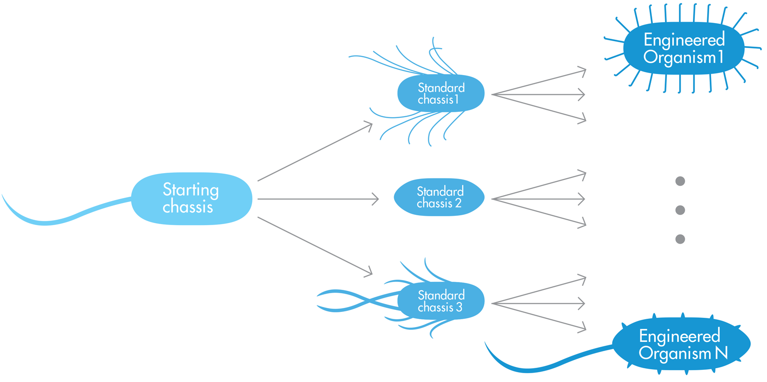
The second approach to chassis design begins with what we’ll call a “standard chassis.” In this approach, shown in Figure 9-2, a synthetic biologist might choose a more generic chassis that either has a minimal number of natural components or is well understood and highly engineerable. The simple chassis essentially provides a blank canvas for the synthetic biologist and could at least theoretically be an ideal chassis for a variety of engineered systems with completely different desired outputs. Taking the standard chassis approach, researchers at Ginkgo Bioworks are using engineered E. coli to make biofuels. Unlike the previous example we considered, in which biofuel production started with R. eutropha, a natural polymer factory, E. coli have no existing talents to recommend them for biofuel production. However, E. coli are the closest organism that the field has to a standard bacterial chassis. Thus, the researchers at Ginkgo Bioworks see E. coli as an attractive platform for many purposes, including the conversion of carbon dioxide and electrical energy into isooctane, a liquid fuel that fits well into the existing transportation fuel infrastructure in the United States.
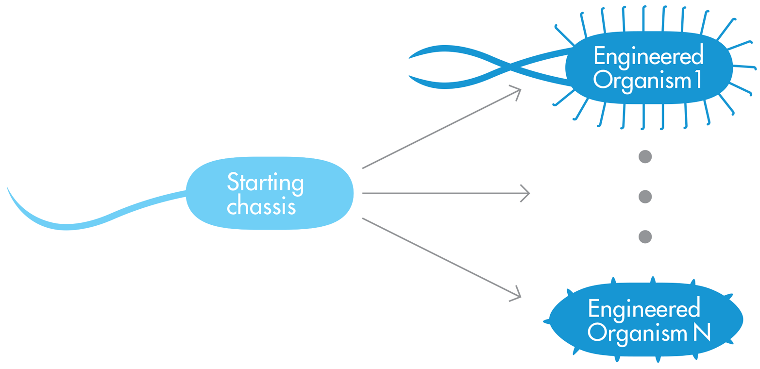
Figure 9-2. The “standard-chassis” approach. The standard starting chassis is simple and easily engineered, so synthetic biologists can use it as a precursor for Engineered-Organism 1, Engineered-Organism N, and everything in between.
Both the nearest wild-type organism and the standard-chassis approach have benefits and drawbacks. For example, if only minor changes are needed in an existing organism to obtain the desired outcome, it might be relatively easy to use the nearest wild-type organism approach. This strategy, however, can be difficult to scale because, for each new design specification, the designer needs to find a new chassis. In addition, using an existing organism as a chassis can be unexpectedly complicated because all organisms have their own metabolic pathways and needs, any of which might interfere in surprising ways with the desired output.
The standard-chassis approach avoids some of the complications that arise when using complex organisms to build synthetic living systems. This approach is also more scalable than the nearest wild-type organism approach because it provides a generic starting point for designers. With a common standardized chassis, designers can reuse the tools for one design for another, at least to some extent. The pie-in-the-sky hope is for a “blank canvas” cell that could be programmed to produce a medicine, food, tissue, or biofuel, but currently this hope is quite far-fetched. For now, cells cannot be abstracted into an agnostic canvas for running DNA programs.
Synthetic biologists, though, are encouraged by the success seen in computer programming for which such cross-platform tools do exist. For example, software platforms such as Java define a “virtual machine” that makes it possible for programs to run on any operating system. The Java virtual machine adapts the Java bytecode so that it works the same way regardless of the operating system. In this analogy, the Java bytecode is analogous to the DNA sequence, and we can think of the Java virtual machine (plus the operating system) as the cellular machinery that converts that code to action. In other words, we can think of synthetic biology’s standard chassis as the Java virtual machine for biology.
It is not yet realistic to imagine one standard chassis for every synthetic biology application, though, so a compromise is being struck between the nearest wild-type and the standard-chassis approaches. In this compromise, a small menu of chassis would serve as a starting point for synthetic biologists, who might choose from a handful of different cell types for any given application area. In this scenario, there might be one or two reliable standard chassis for bacterial applications and another one or two for genetic programs to be run in mammalian cells. Although this is still under development, this hybrid approach to the engineering of cellular chassis is perhaps more likely to yield accessible tools for synthetic biologists to succeed in the near term.
Safety, and How to Engineer It
You must always consider safety when choosing a chassis for running engineered DNA programs. Specifically, researchers must consider their personal safety in working with synthetic living systems, the safety of their lab environment, and any harm that might occur if their engineered organisms enter the wider world.
Existing guidelines and regulations largely protect the personal safety of the researchers and the lab communities where they work. These regulations came into existence in the 1970s with the advent of recombinant DNA technologies. They are generally considered a success, but they were hotly debated at the time, and the debates provide many relevant lessons for synthetic biology today. See the Fundamentals of Bioethics chapter for a more detailed explanation of the guidelines and their development.
In addition to the regulatory work that’s been inherited from the field of genetic engineering, synthetic biologists must carefully consider the safe introduction of synthetic living systems into our complex environment. Ideally, there should be a general approach to minimize and contain any potential damage from organisms that might either escape or are intentionally deployed to the environment outside a lab. Because they carry additional genetic burdens, most synthetic organisms have decreased fitness relative to their natural competitors, which already decreases the likelihood that the engineered organisms will either persist or cause significant damage in the wild. It seems unwise, however, to rely on this inequality, and additional safety measures are being designed as synthetic biologists plan their systems.
Instead, synthetic biologists are trying to engineer for safety. One radical example of “safety by design” is the synthetic biology research to engineer orthogonal DNA that is decoded differently from naturally occurring DNA. Because DNA can transfer between organisms and such transfer is relatively common, there is concern about the potential consequences if an engineered organism were to take up DNA from a naturally occurring organism, and vice versa. However, if engineered organisms were expressing orthogonal DNA that can’t be decoded properly outside the original host, these possible dangers are minimized. Any chassis that uses the altered genetic code couldn’t implement a new—and potentially dangerous—genetic function that it acquired from the outside environment, and the genes from the engineered organisms couldn’t be implemented if they were to be transferred to naturally occurring organisms.
Synthetic biologists are still in the early phases of such research, but a paper published in Science in 2011 showed some promising results. The research group, led by Dr. George Church’s lab at Harvard, “re-coded” E. coli by replacing all of the TAG stop codons they found in the 4.6 million base pair genome with synonymous TAA stop codons, as illustrated in Figure 9-3. Incorporating this seemingly “silent” set of changes was a technical tour de force that motivated the team to develop new, highly useful genome manipulation tools called “MAGE” and “CAGE.” More relevant to this discussion, though, is the fact that the resulting chassis had two safety advantages over the natural bacterial strain. First, all of the coding sequences in the new strain can still be transcribed and translated but because none of them used the TAG codon, that codon can be repurposed to add alternative amino acids to a novel DNA program. The new organism could then be designed for safety by making it reliant on some nonnatural amino acid provided by the researcher but not by nature. Second, the TAG codon is no longer functional as a stop codon in the recoded E. coli because the Church research group also deleted the release factor that terminates translation at any TAG. Therefore, if the reengineered bacterium picks up any external DNA that uses the TAG stop codon, the resulting polypeptide chain will be nonfunctional because the ribosome will continue reading past the stop codon. Further work must be done to make engineered DNA truly orthogonal to naturally occurring genetic material, but this early success in “safety by design” is a nice model to consider as the efforts move forward.
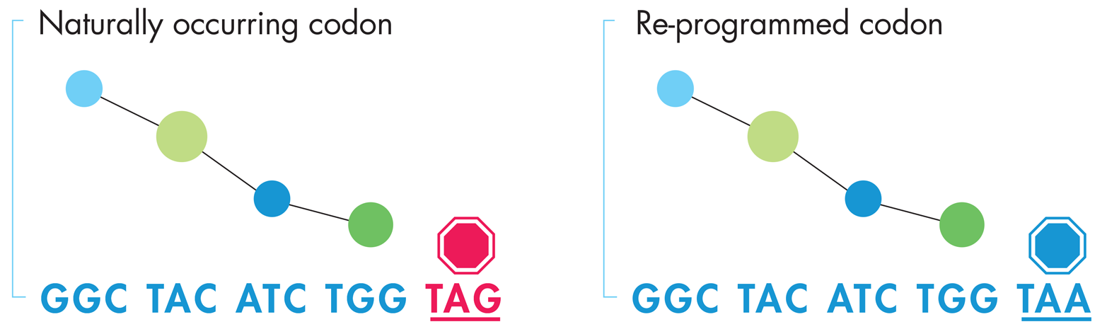
Figure 9-3. One approach to generating orthogonal DNA. The naturally occurring DNA sequence on the left codes for four amino acids, represented by the blue and green balls above the sequence, ending with a TAG stop codon. By converting the DNA’s naturally occurring TAG stop codons (left) to TAA stop codons (right) the protein product is unchanged but the cells expressing this genetic code can be reengineered toward an orthogonal genome by reassigning the TAG codon to an unnatural amino acid.
Background on the E. chromi iGEM Project

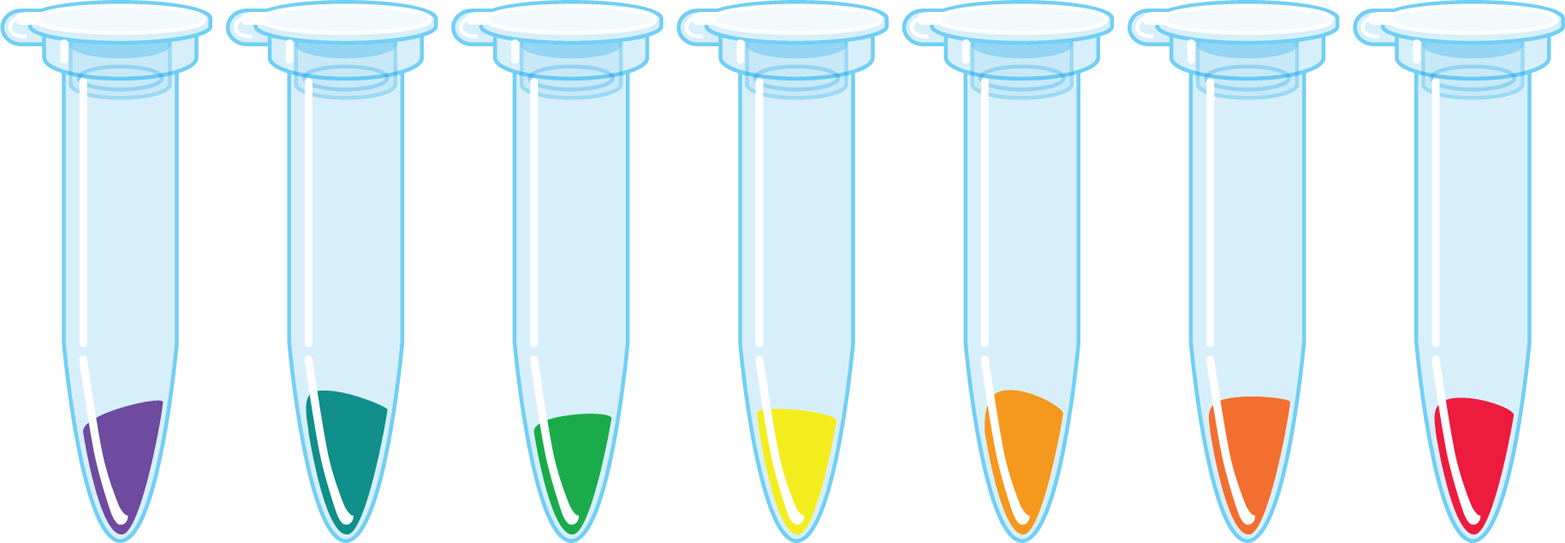
For its iGEM project in 2009, the University of Cambridge team designed, specified, and built a set of biosensors that the team called E. chromi. Given the wide variety of natural colors to be found in the living world (orange carrots, purple flowers, and so on), the team decided to use color as the output for its system. It also decided to make sensors for particular metal compounds, including arsenic, mercury, and other heavy metals that are persistent contamination concerns in some countries. These environmental contaminant inputs would trigger pigment-based outputs visible to the naked eye for easy, immediate deployment. This design was an improvement on previous iGEM biosensor projects that had used outputs such as pH, electrical conductance, and fluorescence, and so required additional steps to detect the output signal. The pigments also offer visual diversity, motivating the team to build a living “dipstick” that could colorfully report on multiple contaminants with one sample swab, as demonstrated in Figure 9-4.
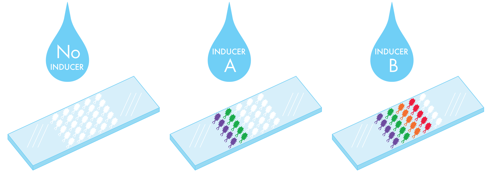
Figure 9-4. Dipsticks that report on multiple contaminants in a single water sample. The dipstick would be spotted with bacteria expressing different genetic programs that sense contaminants and generate color in response. When exposed to water without any inducers (left), no color would be generated. When exposed to water with a mixture of two contaminants (center), the two corresponding colors would be produced. If the water contains four contaminants (right), four colors would be produced.
In addition to detecting the presence of particular contaminants, the team thought it would be useful to approximate the concentration of each contaminant. By developing a collection of “tuner” devices that control the sensitivity of the system, the team could generate variants of each color-generating system so that the system changed color only when a contaminant was present in a specific concentration range. A water sample that has a low concentration of arsenic would trigger only the low-sensitivity tuner and pass that signal to the color-generating device in that variant only. A water sample with a high concentration of arsenic would trigger the low, medium, and high sensitivity tuner and would trigger color in all three variants. With its final system (Figure 9-5), the team could expose its collection of variants to a water sample, and based on which variants produced color and which did not, determine which contaminants were present and at what concentration.
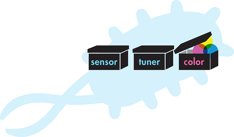
Figure 9-5. System-level design for a living biosensor. The black-box design idea for a cell that is built to detect environmental contaminants and report on their concentration.
About Their Devices

To find DNA sequences that encode bright colors, the iGEM team mined the literature and ultimately identified three naturally occurring bacterial systems that produce unique pigments. These systems are shown in Table 9-1.
|
|
|
Table 9-1. Natural sources for living color production |
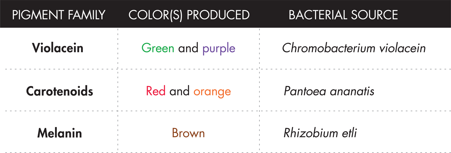
Because the team wanted a variety of colors, it pursued all of these sources as potential devices and found that some were more suitable to certain applications. For example, the melanin pigment is encoded by a single gene, which makes the output relatively easy to control with established gene regulation approaches, but the system also requires that both copper and tyrosine be added to the media, complicating any growth conditions for a strain expressing this color. The other two pigment families are generated through the action of multiple gene products, making their regulation more complex, but cells producing these pigments are simpler to grow because the colors are generated without any unusual compounds in the growth media.
To deploy the system’s devices, the iGEM team also had to consider the distinct mechanisms used to produce the violacein and the carotenoid pigments. The carotenoid devices use a pathway that produces a red pigment first and then uses a downstream enzyme to convert some fraction of the red pigment to an orange one. By contrast, the violacein devices rely on a branched metabolic pathway to produce both green and purple colors, as depicted in Figure 9-6.
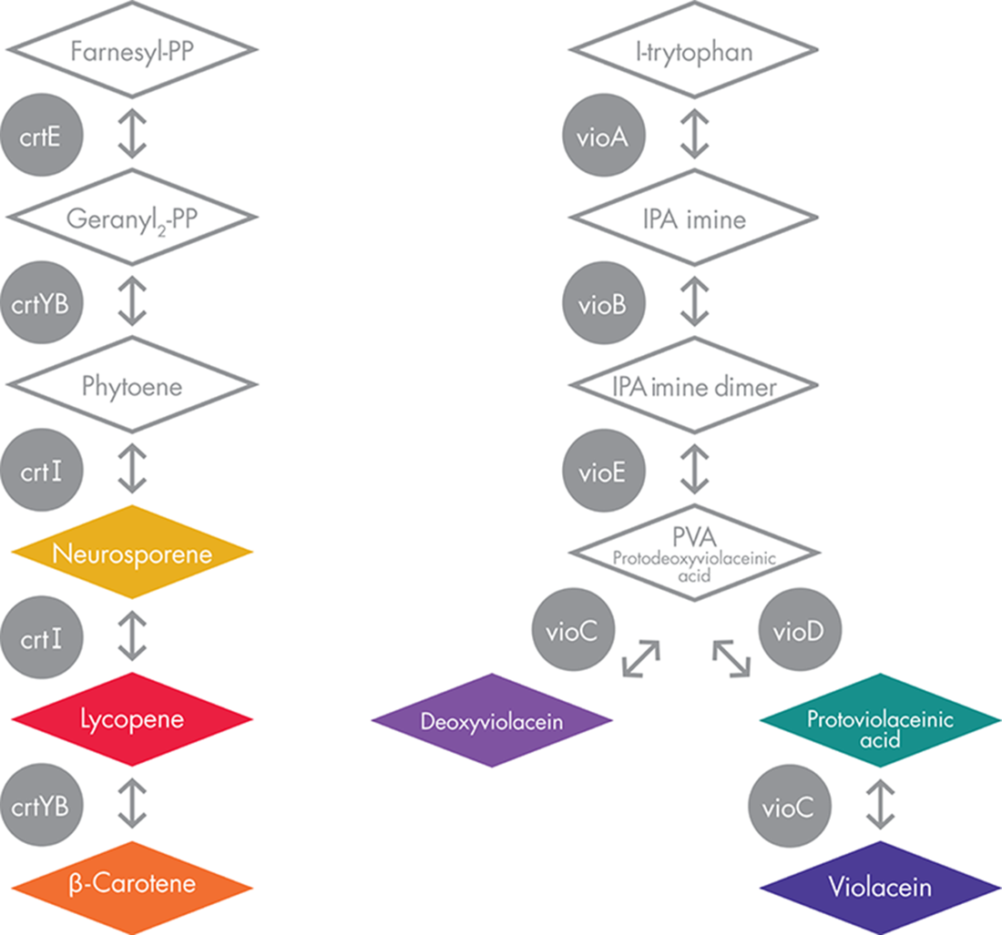
Figure 9-6. Pigment-generating metabolic pathways. The carotenoids pathway is shown on the left, and the violacein pathway on the right. The diamonds represent different cellular intermediates, and the circles represent the enzymes responsible for the chemical reactions. Colored compounds are illustrated in their approximate color.
Parts and Devices
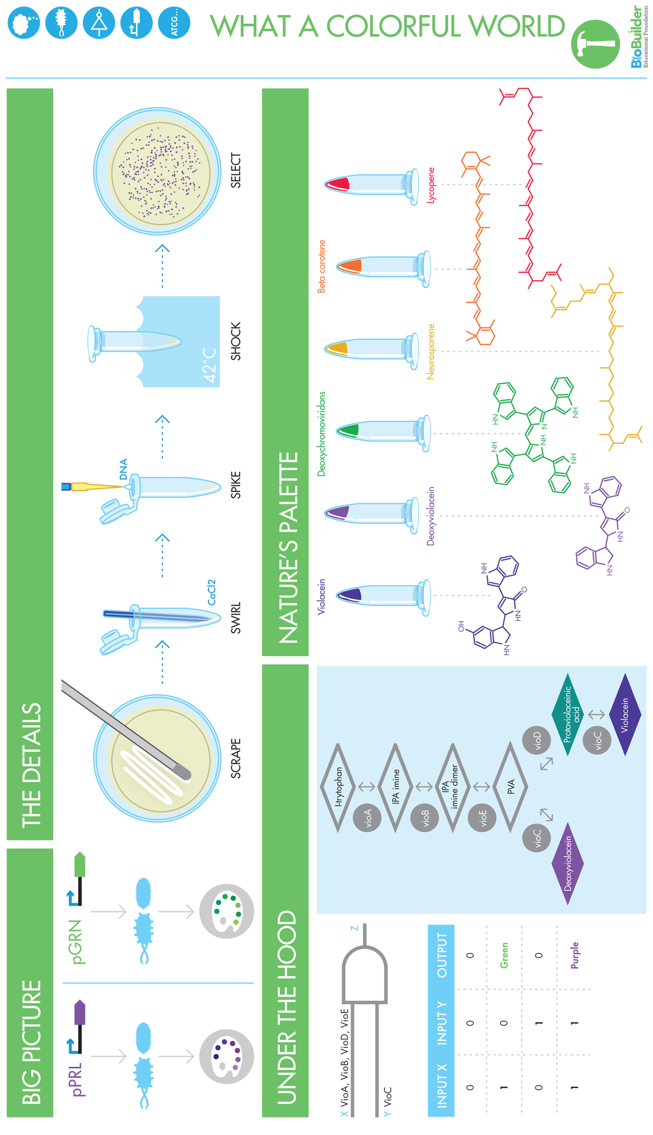
The BioBuilder Colorful World activity uses components from the violacein system that can produce either green or purple pigment, depending on a relatively small genetic change. Normally the input to this pigment-producing system is the amino acid tryptophan and, through the action of five enzymes (VioA, VioB, VioC, VioD, and VioE, but not in that order!) a purple pigment called violacein is produced. When the vioC gene is removed, however, the pathway branch is blocked and the final transformation to violacein can’t occur, so the system’s endpoint instead becomes protoviolaceinic acid, a pigment with a dark green color. You can infer this effect of removing the vioC gene by inspecting the metabolic pathway (Figure 9-6). This behavior can also be illustrated using the engineering formalisms of logic gates and truth tables, as shown in Figure 9-7.
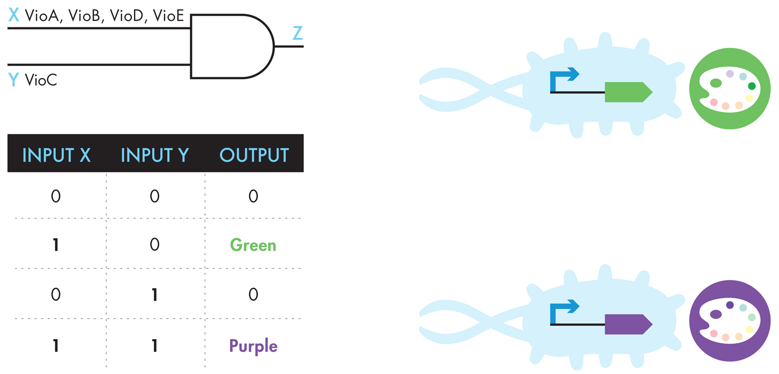
Figure 9-7. Different representations of the violacein-related systems. The logic-gate representation (upper left) shows how input X (VioA, B, D, and E) and input Y (VioC) must be present to generate purple output Z. The modified truth table (lower left) shows that input X alone can create green output, while input Y alone does not generate output, and input X and input Y generate purple output. The genetic schematics to the right show that a promoter upstream of a green-generating device, which consists of VioA, B, D, and E, creates green pigment, and a promoter upstream of the purple-generating device, which consists of VioA, B, C, D, and E, creates purple pigment.
Additional Reading and Resources
§ Changhao, B. et al. Development of a broad-host synthetic biology toolbox for ralstonia eutropha and its application to engineering hydrocarbon biofuel production. Microbial Cell Factories 2013;12:107.
§ Ginkgo Bioworks Foundry (http://ginkgobioworks.com/foundry/).
§ Lajoie, MJ. et al. Genomically recoded organisms expand biological functions. Science 2013;342(6156):357-60.
§ E. chromi website (http://www.echromi.com/).
What a Colorful World Lab
In this lab, bacterial transformation techniques will be used to introduce some plasmid DNA into two cell types. The engineering concept of chassis is explored by comparing the function of identical genetic programs in two different strains of E. coli. Sterile technique and solid-state microbial culture are the biotechnology skills emphasized in this lab.
Design Choices
In our discussion of the E. chromi project, we saw that the iGEM team made some assumptions about the system’s performance. In particular, the team members presumed that the color-generating devices would predictably generate a visible palette of colors when exposed to a given concentration of metal contaminants. The team realized, however, that there were idiosyncrasies for each pigment-generating device. The melanin pigments, for example, require supplemented media. To address these idiosyncrasies, it experimented with a number of bacterial strains, aiming to find the “best” one for running each device.
In this lab, you will pick up this aspect of the iGEM team’s project. You will compare two color-generating devices in two different chassis to investigate whether reliable color output is attainable.
Experimental Question
You will test the purple and the green color-generating devices in two common laboratory strains of E. coli: a K12 strain and a B strain. Both of these strains are routinely used to study the behavior of bacterial cells and to perform molecular biology techniques. They have existed in laboratory environments for so long that they have acquired mutations in many genes that are no longer required for them to survive outside of a narrow set of conditions. As a result, they have all but lost the ability to thrive outside the laboratory environment. Given this description of these cells, they seem to offer the beginnings of the standard chassis for bacterial synthetic biology, at least regarding safety concerns. In this lab, you will investigate whether they are also close to achieving the “utility” requirements for a standard chassis by testing whether they produce reliable, reproducible behavior.
To perform this experiment, you will transform the genetic program that carries the purple and green color-generating devices into each bacterial strain (Figure 9-8). The steps involved in this process include patching the strains to grow the cells you’ll need, and then treating the cells with a salt solution so that they become competent to take in DNA. You will mix your competent E. coli strains with the DNA encoding the color-generating devices, and then you’ll expose the cells to a high temperature for a brief period of time. This heat shock helps the cells take up DNA from the environment. In the final experimental step you’ll add some fresh media to your transformation mixes to help the cells recover, and then you’ll finish by plating the transformed cells onto Petri dishes filled with agar-solidified media that also contains the antibiotic ampicillin. The DNA that encodes the color-generating devices also encodes the ampicillin resistance gene, so the only cells that can grow on the plates are those that have the color-generating device.
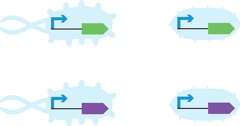
Figure 9-8. Color-generating devices in different chassis. You will insert identical devices into different chassis (left versus right) and investigate their behavior.
As a negative control, you will include a sample that does not contain plasmid during the transformation procedure. This negative control is not expected to grow on the ampicillin-containing plates, because it does not contain the ampicillin-resistance gene. If growth is observed, you know there is something about your procedure or materials preventing the selection of only cells that have been successfully transformed with plasmid. One potential reason might be that the ampicillin in your plates has degraded over time. Including controls is crucial for good experimental design, because it makes it possible for you to isolate variables and can inform any future attempts to troubleshoot problems encountered while doing experiments.
The data you collect will be based on visually inspecting the plates—your eye is the only fancy detecting device you need. After one night of growth, each cell that survived the transformation and antibiotic exposure will have had time to grow into a colony of cells visible to the naked eye. You will count the colonies to determine your transformation efficiency, and you will note the color, shape, and size of the colonies on the different plates to determine whether the strain chosen as the chassis affects the system’s output.
Getting Started
The two plasmids that are compared in the What a Colorful World experiment are detailed in Table 9-2.
|
Plasmid |
Registry plasmid # |
Plasmid description |
|
pPRL |
BBa_K274002 |
pUC18 plasmid backbone, AmpR |
|
pGRN |
BBa_K274004 |
pSB1A2 plasmid backbone, AmpR |
|
Table 9-2. What a Colorful World plasmid and strain descriptions |
||
4-1: NEB E. coli K12 ER2738: F’proA+B+ lacIq Δ(lacZ)M15 zzf::Tn10(TetR)/ fhuA2 glnV Δ(lac-proAB) thi-1 Δ(hsdS-mcrB)5
4-2: NEB E. coli BL21 C2523: fhuA2 [lon] ompT gal sulA11 R(mcr-73::miniTn10--TetS)2 [dcm] R(zgb-210::Tn10--TetS) endA1 Δ(mcrC-mrr)114::IS10
This lab requires two strains of E. coli: 4-1 (K-12 type) and 4-2 (B type). To obtain sufficient amounts of bacteria to carry out the transformation, you will need to replate these colonies as patches. Each patch will provide sufficient bacteria for one lab group, and up to six patches will fit comfortably on one plate.
1. Using a sterile inoculating loop or toothpick, transfer a bacterial colony from one of the Petri dishes to a new Luria Broth (LB) agar (NOT LB+amp) Petri dish, drawing a 1 cm x 1 cm square of each strain. Each square you draw this way will yield enough cells to transform with two plasmids.
2. Repeat for each strain you will need for the transformation lab.
3. Place Petri dishes in the incubator at 37°C overnight.
Lab Protocol
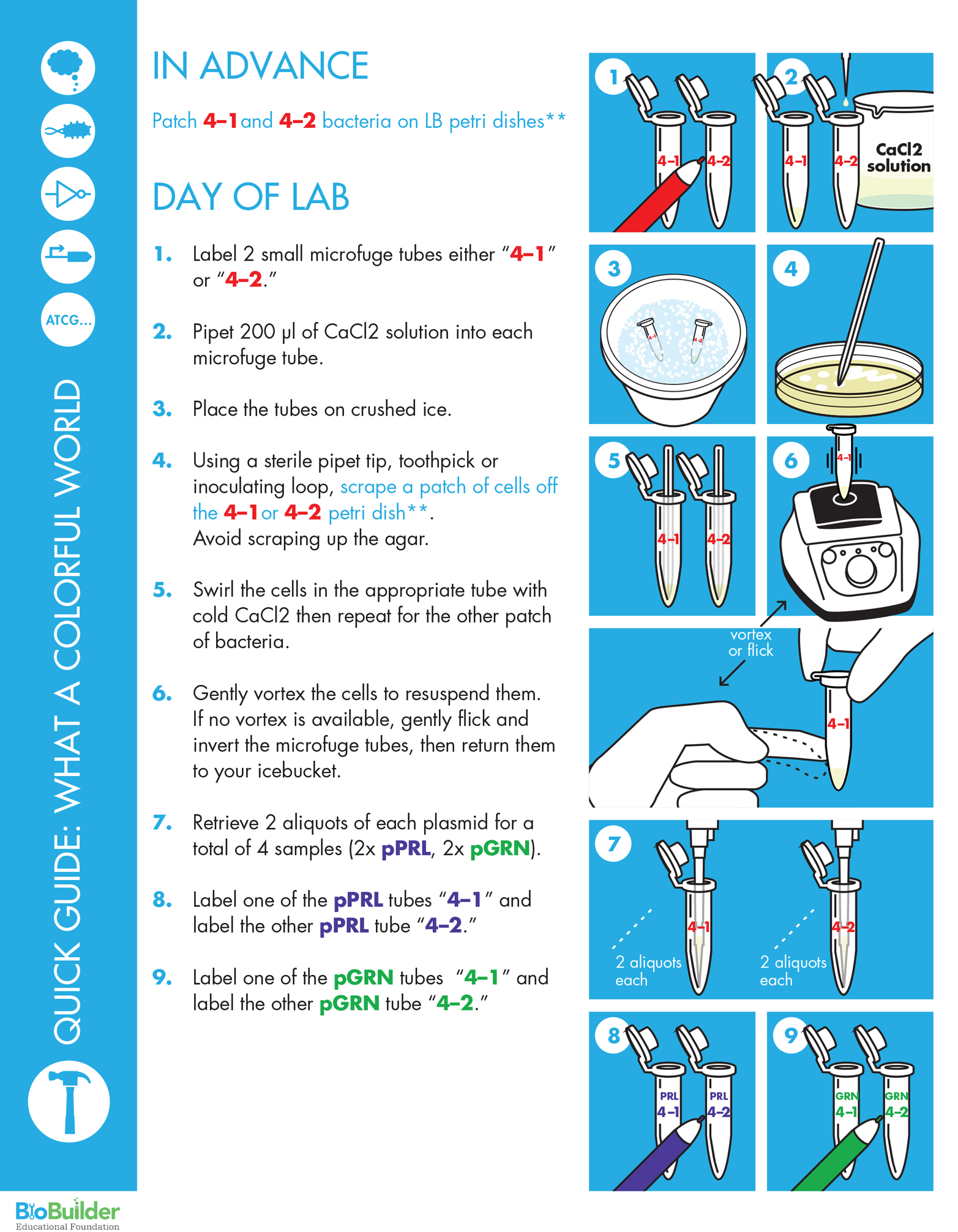
1. Label two small microfuge tubes “4-1” and “4-2.”
2. Pipet 200 μl of CaCl2 transformation solution into each tube and then place the tubes on ice.
3. Use a sterile wooden dowel or inoculating loop to scrape up one entire patch of cells (NOT including the agar that they’re growing on!) labeled “4-1,” and then swirl the cells into its tube of cold CaCl2. A small bit of agar can get transferred without consequence to your experiment. If you have a vortex, you can resuspend the cells by vortexing for one minute. If no vortex is available, gently flick and invert the tube.
4. Repeat, using a different sterile wooden dowel to scrape up the patch of cells labeled “4-2.” Vortex briefly if possible. It’s okay for some clumps of cells to remain in this solution.
5. Keep these competent cells on ice while you prepare the DNA for transformation.
6. Retrieve two aliquots in microfuge tubes of each plasmid for a total of four samples (2x purple-generating device plasmid, pPRL, 2x green-generating device plasmid, pGRN). Each aliquot has 5 ul of DNA in it. The DNA is at a concentration of 0.04 μg/μl. You will need these values when you calculate the transformation efficiency at the end of this experiment.
7. Label one of the pPRL tubes “4-1.” Label the other pPRL tube “4-2.” Be sure that the labels are readable. Place the tubes in the ice bucket.
8. Label one of the pGRN tubes “4-1.” Label the other pGRN tube “4-2.” Ensure that the labels are readable. Place the tubes in the ice bucket.
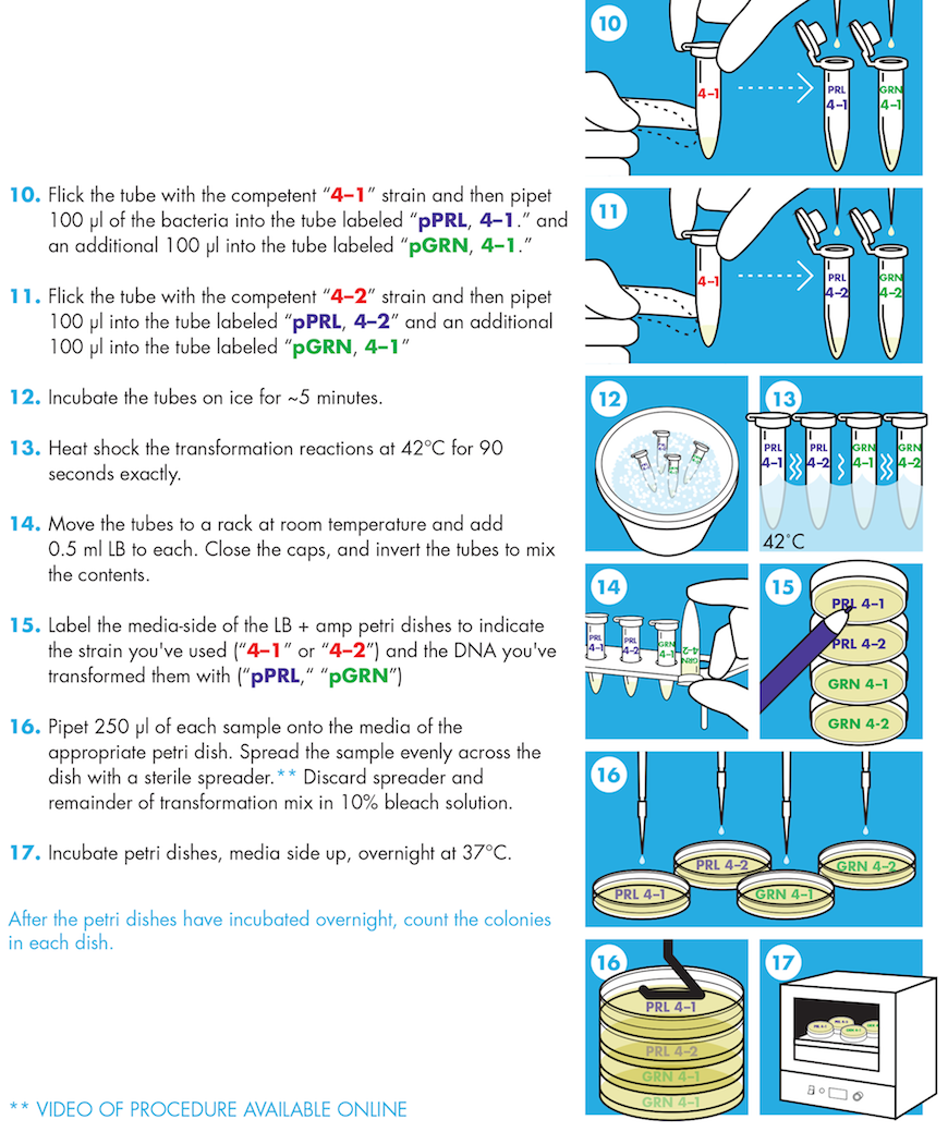
9. Flick the tube with the competent 4-1 strain and then pipet 100 μl of the bacteria into the tube labeled “pPRL, 4-1” and an additional 100 μl into the tube labeled “pGRN, 4-1.” Flick to mix the tubes and return them to the ice. Save the remaining small volume of the 4-1 strain on ice.
10.Flick the tube with the competent 4-2 strain and then pipet 100 μl into the tube labeled “pPRL, 4-2” and an additional 100 μl into the tube labeled “pGRN, 4-2.” Flick to mix and store them, as well as the remaining volume of competent cells, on ice.
11.Let the DNA and the cells sit on ice for five minutes.
12.While your DNA and cells are incubating, you can label the bottoms (media side) of the six Petri dishes you’ll need. The label should indicate the strain you’ve used (“4-1” or “4-2”) and the DNA you’ve transformed them with (“pPRL,” “pGRN,” or “no DNA control”).
13.Heat shock all of your DNA/cell samples by placing the tubes at 42° for 90 seconds exactly (use a timer).
14.At the end of the 90 seconds, move the tubes to a rack at room temperature.
15.Add 0.5 ml of room temperature LB to the tubes. Close the caps, and invert the tubes to mix the contents.
16.Using a sterilized spreader or sterile beads, spread 200-250 μl of the transformation mixes onto the surface of LB+ampicillin agar Petri dishes.
17.Cover the plate and set aside for a minute. Then, turn the plate over. The plates will be stored upside down to prevent condensation from dripping onto the bacteria.
18.Incubate the Petri dishes with the agar side up at 37°C overnight.