BioBuilder: Synthetic Biology in the Lab (2015)

BioBuilder’s iTune Device activity emphasizes the “test” phase of the design-build-test cycle. You will be working with several variants of an enzyme-generating genetic circuit. The circuits have small differences in their DNA sequences, which are expected to change the amount of enzyme the cells produce. You will use an enzymatic assay to quantitatively measure the circuits’ outputs. You will then compare your results with what you would predict based on the known behavior of the slightly different DNA sequences.

For most engineered systems, significant differences between observed and predicted behavior are unacceptable. As is pointed out in Figure 7-1, what would an aeronautical engineer think of a new wing shape which, when added to the body of an airplane, made the plane fly in unexpected ways? Designing and building in the face of such uncertainty would create huge expense and potentially put lives in danger. Engineers would find it nearly impossible to move forward with their designs if the combinations of simple parts—be they nuts and bolts or resistors and amplifiers—gave rise to unexpected behaviors.

Figure 7-1. Unintended behaviors. In modifying the standard tail of an airplane (left) to a novel shape (right), the engineer must be concerned about unintended behaviors, for example differences that affect how the airplane can land safely.

More established engineering disciplines rely on modular components that can be functionally assembled in a variety of ways, making it easy to customize combinations according to an individual’s needs. The pieces not only need to be physically connected but, when connected, they also must behave according to specification. To put it simply, the parts must function as expected when they are assembled.

At this point in the field of synthetic biology, biological engineers are still working toward such functional assembly of genetic parts. Even though researchers have characterized many cellular behaviors at the molecular level—and in many cases it’s possible to catalog the genetic elements necessary and sufficient to carry out a biological function—combining these genetic components in new ways often generates unexpected results. Synthetic biologists might soon be able to physically assemble the genetic material to assemble any desired sequence relatively easily, but placing that sequence in a new cellular context can affect its function in uncertain and changing ways, even if the sequence has been thoroughly studied and well characterized in isolation or in other contexts.

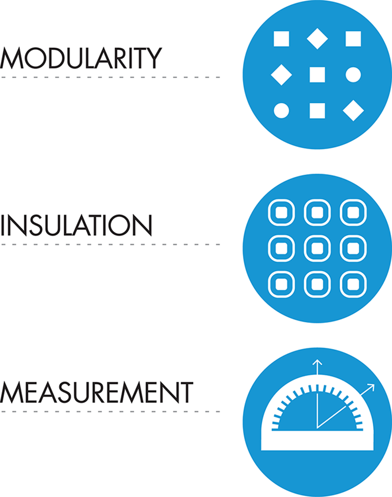
Modularity, insulation, and measurement of parts are crucial components toward enabling such functional assembly, in addition to standardization (see the Fundamentals of DNA Engineering chapter for further discussion). In this chapter, we explore how these additional principles are applied in standard engineering in general and synthetic biology in particular. Then, we detail the iTune Device experiment to test a variety of genetic circuits in cells, in order to compare their expected and their measured behaviors.

Modularity

Modularity refers to the idea that engineers can design and generate systems by combining functional units, or “modules.” As intuitive as this notion is for engineering, the idea of modularity has only recently been applied to genetic parts. Modularity is sensible to apply to biology because we can attribute discrete functions to particular snippets of DNA—however, even though we take this principle for granted now, significant research was required to confirm it (see the following sidebar).

GENES AS MODULES

Synthetic biology assumes a set of genetic “parts” that can be combined and manipulated to generate precise behavior. The idea underlying this premise—that traits arise from discrete functional bits of DNA—is in fact relatively new. It was not until the results from Gregor Mendel’s experiments with pea plants were rediscovered in the early 1900s that scientists began to understand that traits could remain distinct, paving the way for our current understanding of genetics.

For a long time, offspring were thought to blend the genetic traits from parents. Mendel’s meticulous work breeding pea plants showed that blending did not always occur, and that sometimes a trait can be faithfully passed from a parent plant to an offspring plant. Mendel conducted these inheritance studies by carefully counting and measuring some key traits of his pea plants, such as flower color and pod shape. His data showed that traits could remain distinct and were handed down independently in predictable ratios. His results suggested that heredity should be considered in terms of discrete entities, which he called factors but which were later named genes. His work showed how these factors passed in predictable ways between generations. This idea is taken for granted today, but it was groundbreaking in its time, leading to the founding of the field of classical genetics.

It took more than 50 years to provide a molecular explanation for the inheritance patterns that Mendel observed. Our modern understanding relies largely on DNA’s double-helical structure, as described by Watson and Crick, and on the classical studies of gene expression in the lac operon from Jacob and Monod. Thanks to these scientific advances and others, we now understand foundational ideas in biology, such as the flow of genetic information from DNA through RNA to proteins and the recasting of traits as DNA sequences that encode a function. The idea of DNA parts in synthetic biology is a product of these classical achievements.

Changes in the recorded music industry offer a decent (but not perfect) example of the advantages gained from increased modularity. For much of the twentieth century, the most common, and profitable, way to distribute music was as records and, later, as cassette tapes and CDs. In all of these formats, music was sold primarily as full-length albums. Single songs were available but were significantly more costly, so even if people only liked a few of the songs on an album, they generally bought the album. The album was the standard “unit” for the music industry and its artists. This unit changed completely in the early twenty-first century, when music was digitized. With this advance, it became easy to download music instead of buying the physical album. Songs from an album were easily unbundled, making songs independent modules that listeners could mix and match as desired and needed. The widespread opportunity to make customized playlists from these modular songs has changed the way people think about their music collection and has altered the standard “unit” for the industry.

The enhanced modularity and customization we see in commercial music recapitulates our changing notions of a gene expression unit, which have paved the way for the use of the term genetic “parts” in synthetic biology. Mendel’s early work showed that traits were discrete entities. In the analogy with recorded music, then, the organism displaying the trait can be considered analogous to the full album—the trait only exists in the context of the organism, just as the song only exists in the context of the full album. Dr. Francois Jacob and Dr. Jacques Monod, whose work is detailed later in this chapter, dramatically recast this picture with their description of lactose metabolism, reframing traits in terms of dynamic genetic elements rather than whole organisms with traits. Particular stretches of DNA were identified that worked in concert to control a cell’s behavior, but the genetic elements within those stretches were indivisible and not easily customized to meet a new purpose. This landmark can be considered somewhere between the “album” and “single” phases of the music industry. Now, in the era of genetic engineering and interchangeable genetic parts, many genetic sequences encoding specific functions are known and can be precisely manipulated. We can customize a “playlist” of these genetic elements by recombining them in specialized ways to suit our needs. The techniques for this manipulation are more fully described in the Fundamentals of DNA Engineering chapter. Here, we’ll explore the engineering opportunities that arise because we can mix-and-match genetic parts.

Insulation

As modular materials are mixed and matched, new complications arise, including the increased chance that the modules can interact with one another in undesirable ways. One tool to minimize unanticipated interactions between modules is to insulate the behavior of the parts. Consider the modular options available when buying a car. You can upgrade the basic model in many ways: enhanced speaker systems, a more powerful engine, heated rear seats, and more. These add-ons are available thanks, in part (ha!), to the modular design approach that the car’s engineers employed. Without this approach, the cost of upgrading to a fancy speaker system would be exorbitant because the front console would need to be entirely redesigned to accommodate each brand of speakers. Instead, flexibility for snap-in upgrades was included in the early design stages, and consequently changes at the time of purchase don’t require significant redesign efforts. Customization for each of the car’s modules was anticipated, and designers put in the hard work in at the outset to make the parts discrete.

In addition to creating physically discrete parts that can be combined in many ways, functional assembly requires that the parts exhibit behaviors that are separable from the other elements around them. For example, as Figure 7-2 illustrates, the operation of the stereo must not affect the operation of the driver’s steering wheel. It would be a real driving challenge if twisting the knob on the radio also turned the steering wheel. Such behavioral separation between the operation of parts is referred to as insulation.

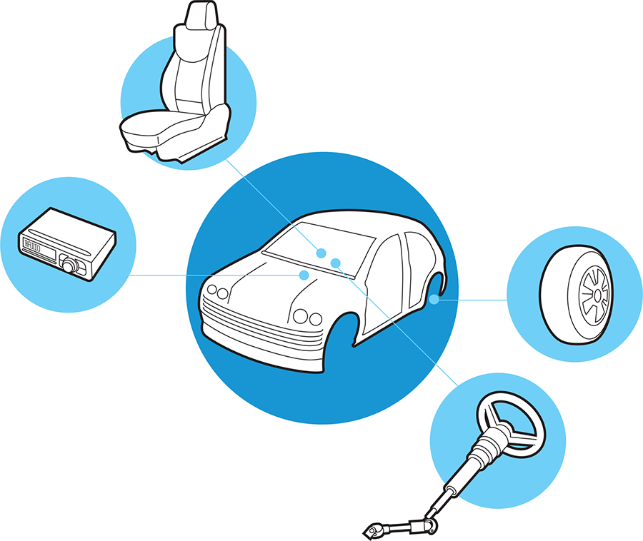
Figure 7-2. Insulation in car design. A modern car consists of multiple components, including the seats, wheels, steering wheel, and stereo. Components work independently, so the use of one component does not interfere with the operation of other components in the car.

Similar anticipatory design and insulation of genetic parts is difficult to achieve when building with genetic parts. The cell is a fluid environment where molecules, proteins, and cellular structures are constantly mixing. How is it possible to insulate their behaviors when they encounter new partners and neighbors all the time? In addition, “upgrades” to a cell might behave as expected in some cellular settings and not as expected in others. The activity in the What a Colorful World chapter exemplifies this challenge. Even if the upgrades seem to work at first, the cell’s local environment is dynamic, requiring that cellular designs operate under many environmental and growth conditions. Finally, unlike any other engineering substrate, living materials can and will mutate over time, as we explore in the Golden Bread chapter. Evolution of the engineered product makes the design challenge that much greater.

To manage all the complexity of biological design, we can use the powerful engineering tool of abstraction, as described in the Fundamentals of Biodesign chapter, so decisions about one design element can be made independently from the decisions made for other elements. A car’s stereo can be swapped without affecting the steering. Moreover, modularity, insulation, and abstraction should allow decisions about devices to be made without having an impact on the system design. Referring back to the automotive analogy, you don’t need to buy a truck instead of a car just because you want front-wheel drive.

But how well does such an approach work for synthetic biology in practice? Synthetic biologists would like to reach a point where they can predictably and rationally combine parts with known identities and relative strengths into new synthetic circuits. By measuring the actual performance of synthetic systems, composed of well-characterized parts, and comparing the measurements to what was predicted, biobuilders can assess their designs and move closer to correctly anticipating the success or failure of future designs.

Principles of Measurement

Some things are hard to measure. Happiness, for example, has no scale or unit that we can all agree on, and there are no instruments to reliably detect it. Other things are measured all the time: we can associate a numerical value to cards in a deck, grade-point average, or team standings in a sports league. Whether you’re cooking a meal or buying clothes off the rack, you rely on measurements to number, size, time, or count things. Measurements report on the state of the items, and their behaviors, relationships, or characteristics.

When something can be measured, units give us a common way to compare items. Standardizing the units for each measurement is not trivial, as we described in the Fundamentals of DNA Engineering chapter, but for many items, there are units on which we have agreed. Measuring the height of a horse in “hands” is a great example. Thanks to Henry VIII, who standardized a hand to 4 inches, even this antiquated unit still has meaningful measurement information. Anyone who is familiar with the hand measurement knows that a horse standing 16 hands high is 64 (16 x 4) inches at the withers (near the shoulder) and that another horse measuring 16.3 hands is 67 (16 x 4 + 3) inches, not 65.2 (16.3 x 4) inches.

Meaningful measurements, no matter the unit, are a hallmark of modern scientific approaches. As Mendel showed us, we can see patterns when we count things. Qualitative data can also be highly informative, as explored in the Eau That Smell chapter. Here, though, we spotlight how mathematical measurements powerfully allow us to manipulate and convert information to other representations. Numbers also make it possible for us to make comparisons and predictions.

As an example, try to compare your walk to school with that of your friend when qualitative measurements are all you have. In such a case, you’re limited to saying things like, “school is very far from my house, much farther than from yours, but I walk faster than you do.” But by measuring the miles, times, and speeds, suddenly it’s possible to figure out how early you each need to leave home to meet at school at 8 A.M. If you know the distances and your walking rates, you can anticipate how long the trip will take. Applying this lesson to engineering: measurement gives us the ability to predict, which can be very useful—but only if we can make relevant measurements. What makes a measurement relevant is described next.

What’s Normally Measured

Engineers use measurement not only to describe but also to control, assemble, and improve the objects being measured. The assembly of modular parts illustrates the importance of measurements. To reliably compose one part with another, the relevant features of each part must be known and must conform to some agreed-upon standard. Otherwise, gears won’t turn, nuts won’t fit on screw threads, and Lego bricks can’t be assembled into models of both the Death Star and the Eiffel Tower. By conforming to particular measurement standards, modular parts became the foundation for modern factories and efficient assembly-line manufacturing. Some of the comparisons and measurements that engineers rely on are detailed in Table 7-1.

Making and Reporting Measurements for Synthetic Biology

What you measure will tell you different things about how synthetic DNA circuits are working in a cell. The most direct measurement of a circuit’s activity would be made if we could shrink down to microscopic size, just as Ms. Frizzle does in the Magic School Bus book series, and then magically sit on the DNA to count the number of RNA polymerases that move along the DNA every second. In electronic terms, this would be like counting electrons as they flow in a current. More experimentally reasonable, however, is to measure the products of transcription and translation. How many mRNAs are made per second or how does the protein accumulate over time? These RNA and protein measurements are possible but intensive in terms of the equipment, time, and expertise needed. To make things a little easier in BioBuilder’s iTunes laboratory activity, β-galactosidase (β-gal) activity is measured, which is an indirect but good reflection of the performance of each circuit.

Experience has shown that when DNA circuits are moved from one biological context to another, it can be difficult to predict how the genetic parts will work. The activity of a part is variably affected at many levels, including the rates of transcription, translation, and protein activity in its new cellular environment. Adding to the challenge of reliable assembly is the fact that, when composing living systems made from multiple genetic parts, it’s difficult to predict how the parts will communicate with one another. For example, a strong “on” signal generated by one part might not be strong enough to trigger a downstream part with which it is intended to work.

Synthetic biology, however, is not the first engineering effort to encounter these assembly challenges. One approach that more established engineering disciplines have employed is to develop data sheets that describe how any given part will work as a function of specific parameters. To make such data sheets, engineers must collect sufficient data to fully describe their part, testing them with particular inputs and under many different conditions and environments.

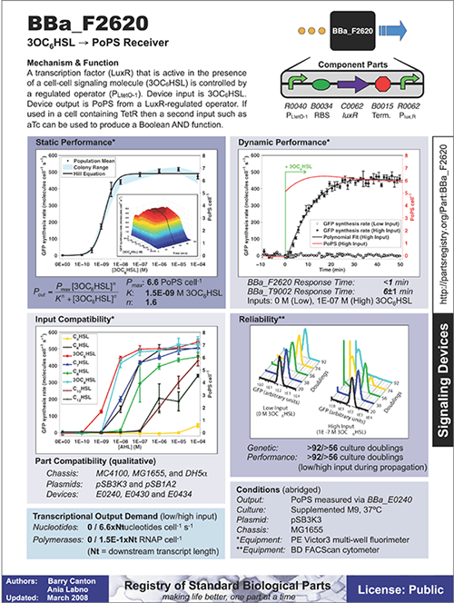
Synthetic biologists can create similar data sheets for their parts. For example, one data sheet that’s been published for a transcription factor in the Registry of Standard Biological Parts reports the part’s static performance, dynamic performance, input compatibility, and reliability. These are the same parameters described earlier in Table 7-1. Ideally these measurements and descriptions of the part’s behavior would hold whenever it is used. However, even if its behavior differs depending on context, the instructions and information on the part’s data sheet might allow a biobuilder to take this variability into account. This “data-sheet” approach only works for parts that vary in reliable and predictable ways, which is not always the case, but it is an important first step toward functional standardization.

Another factor that contributes to a part’s perceived robustness (or lack thereof) is the normal lab-to-lab variability in measurement techniques. Even two people in the same lab who are measuring the same thing are unlikely to come up with identical values due to subtle variations in technique, media, cell growth state, and who knows what else. Synthetic biologists are keen to identify the underlying causes of these variations but appreciate that this is a long-term goal. In the meantime, you can use calibration references to compare measurements made in one place to the measurements made in another. BioBuider’s iTune Device lab makes use of a reference standard for just this reason.

Foundational Concepts for the iTune Device Lab

In this BioBuilder activity, you can explore the biological activity of genetic parts that are expected to work in combination to generate different amounts of an enzyme. Each of these parts has been independently characterized as “weak,” “medium,” or “strong.” This activity asks how well you can anticipate the behavior of these individually characterized parts when they are combined in different ways. Some understanding of gene expression and the role of promoter and ribosome binding site parts, as described next, is essential to begin.

Promoters and RBSs

Often termed the “central dogma” of gene expression, the mantra “DNA makes RNA makes protein” is shorthand for the tenet that proteins are assembled by translation of RNA sequences, and RNA sequences are transcribed from DNA sequences. Proteins carry out many key jobs in a cell, so transcription and translation control many of the cell’s behaviors and traits. Not surprising, then, transcription and translation have been extensively studied, and many of the core components that are necessary and sufficient for controlled gene expression are known (Figure 7-3).

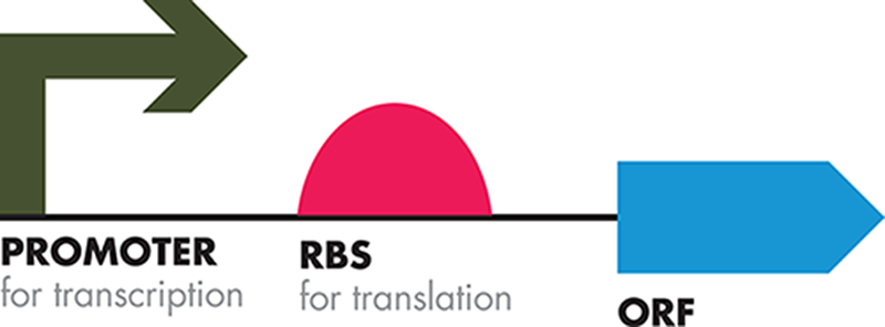
Figure 7-3. Symbolic representation of a gene expression unit. The promoter sequence, represented by the arrow on the left binds RNA polymerase to initiate transcription. The ribosome binding site, abbreviated as “RBS” and represented by a half-circle, is a DNA sequence that encodes the segment of mRNA where the ribosome binds to initiate translation. The open reading frame, abbreviated “ORF” and represented by the arrow on the right represents a DNA sequence that encodes a protein. The direction of the arrows for the promoter and ORF indicate the direction in which they are read.

For transcription, promoters are the DNA sequences that bind RNA polymerase, a complex multiprotein enzyme, to initiate the formation of RNA chains from the DNA template. For translation, the initiation site is termed theribosome binding site (RBS) because the ribosome recognizes this sequence to begin protein synthesis from the RNA template. These sequences are largely responsible for naturally occurring transcription and translation regulation, and synthetic biologists can also use them to introduce their own regulation schemes. Based on the many known promoter and RBS sequences, researchers have identified a consensus sequence for these parts, as demonstrated in Figure 7-4. The consensus promoter sequence, for example, has been determined through a comparison of the nucleotides at each position in many promoter sequences. The consensus is built from the pattern of nucleotides found most often in each position.

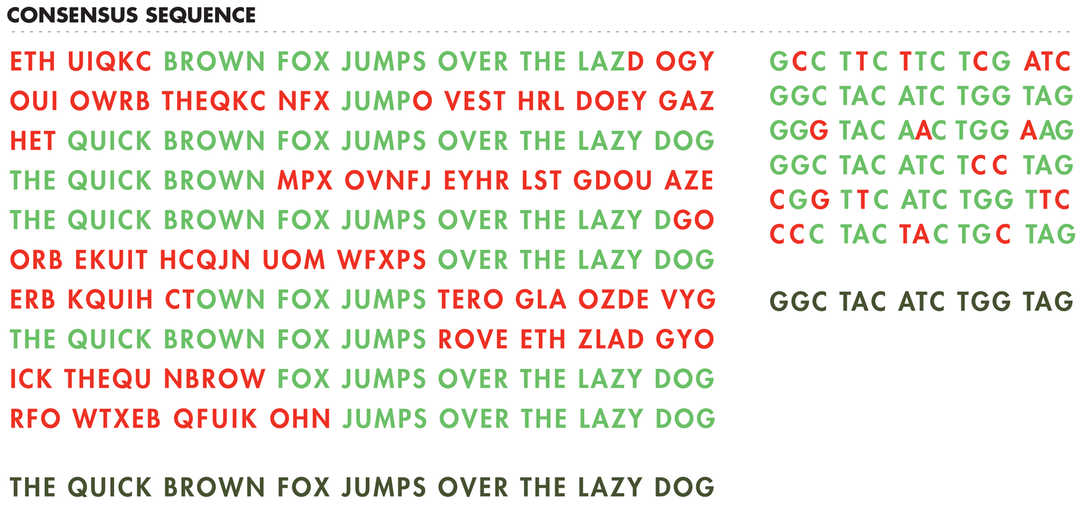
Figure 7-4. Defining consensus sequences. Multiple “sequences” for a sentence (left) and a gene (right) are aligned to generate a consensus sequence, shown in the bottom line in gray. Letters colored green represent the most common letter at each position, which define the consensus sequence. Letters in red are not the most common letters at that position and so are not included in the consensus sequence.

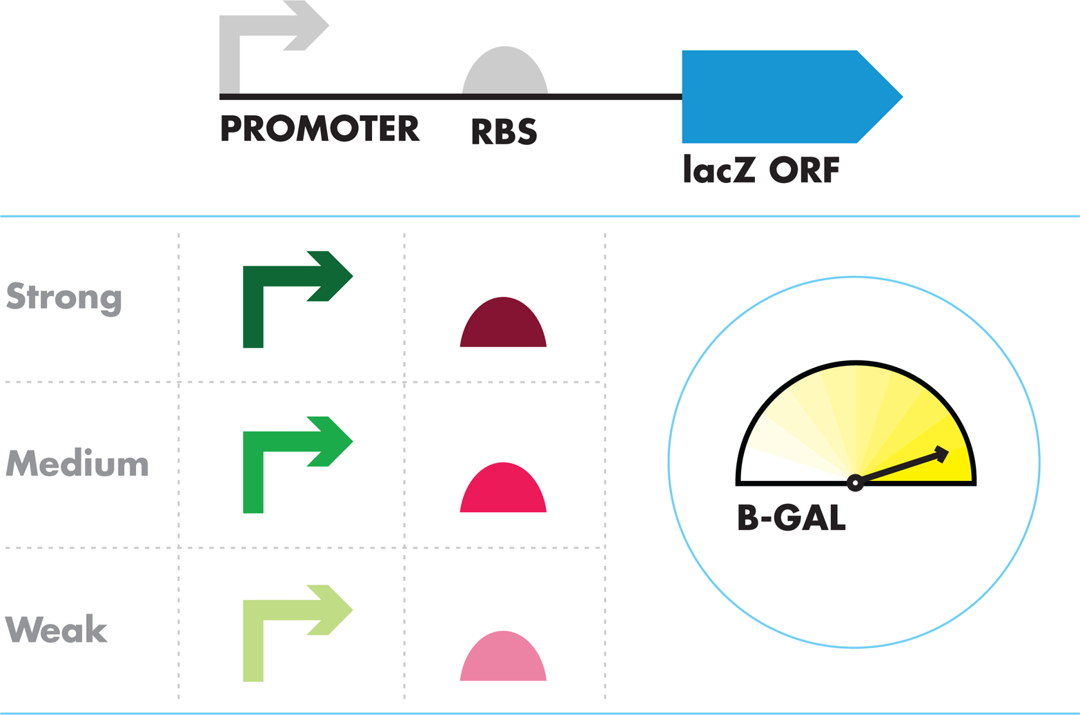
Consensus sequences are relevant for synthetic biology because, generally speaking, a part functions best when it closely matches the consensus sequence. Conversely, the more nucleotides that differ from the consensus sequence, the less capably that part can do its job. Thus a consensus promoter sequence is probably a “strong promoter,” meaning that it will probably bind RNA polymerase well and initiate transcription often, whereas a promoter or RBS sequence that deviates from consensus will be “weak,” doing its job less efficiently than a sequence with better matches. Strong, though, does not necessarily mean better. Depending on the application, an engineer might want only a small level of activity, if, for example, a pore on the cell’s surface were being made or if a cell death response were being regulated.

The Lac Operon

A cell’s ability to turn gene products on and off as needed is critical to its survival. In the 1960s, Dr. Francois Jacob and Dr. Jacques Monod identified foundational principles of gene expression through their studies of lactose transport and metabolism in bacteria. The genes for lactose metabolism are clustered in the lac operon (Figure 7-5), but the bacteria conserve energy by turning on these genes only when glucose is absent. Bacteria prefer glucose as a food source, and will only make the effort to utilize lactose if its preferred food is absent. The molecular details in Jacob and Monod’s explanation for its regulation are a classic model for inducible gene. Here we only discuss the details relevant for the iTune Device lab.

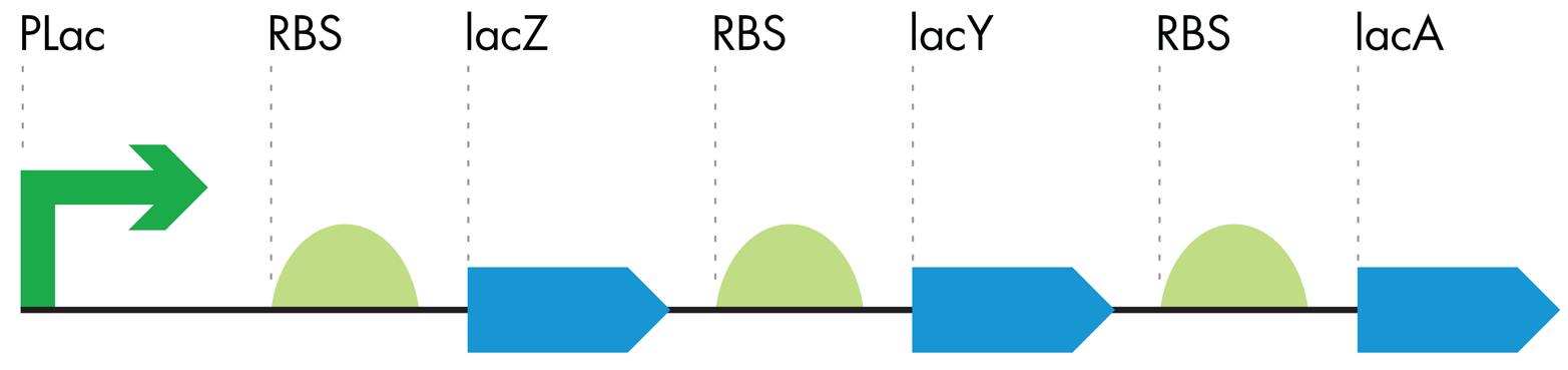
Figure 7-5. Symbolic representation of the lac operon. The lac operon consists of a single promoter (pLac, green arrow) controlling three downstream RBS-ORF pairs (green semicircles and blue arrows, respectively). The operon produces the enzymes necessary to metabolize sugars only when glucose is not present.

The key protein for lactose metabolism is an enzyme called β-galactosidase, often abbreviated β-gal, and it is encoded on the DNA by the ORF called lacZ. The β-gal enzyme cleaves lactose into glucose and galactose, which can be used by the cell to power its other functions. Researchers have also found that β-gal reacts with a variety of molecules similar to lactose, including synthetic analogs such as ONPG, which you will use in the iTune Device lab.

LacZ expression, and that of the entire lac operon, is regulated both positively and negatively at the transcriptional level (Figure 7-6). Positive regulation occurs when a DNA binding protein increases the amount of transcription through DNA elements downstream from its DNA binding site. Conversely, negative regulation is the term used to describe the case in which DNA binding proteins turn down the amount of transcription when they bind the DNA. For the lac operon, the positive and negative regulatory factors are sensitive to the kind of sugar in the bacteria’s environment. When glucose is present, the regulatory factors turn off transcription of the downstream ORFs. If lactose is present and glucose is absent, those same transcription regulatory factors switch their behaviors, and transcription of the operon leads to transport and metabolism of lactose.

The same positively and negatively regulated promoter that controls lacZ also controls the other lac operon genes, including the one that encodes the lactose transport protein. A single mRNA is transcribed from the lac operon’s promoter, giving rise to the multiple protein products needed for lactose metabolism and transport. Translation of each product can occur from the single mRNA thanks to the RBSs that are associated with each ORF. It is a compact and elegant genetic architecture that nature has tuned to produce the needed amounts of each protein when appropriate.

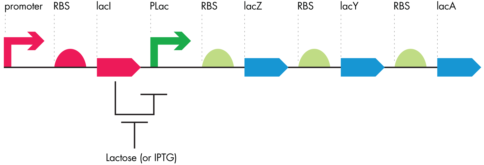
Figure 7-6. Lac operon regulation. The lacI ORF codes for a transcriptional repressor that blocks the P_lac promoter and therefore blocks the expression of the entire operon. Lactose, or its analog IPTG, inhibits the LacI repressor protein, allowing the P_lac promoter to function and relieving inhibition of the downstream operon.

Additional Reading and Resources

§ Canton, B., Labno, A., Endy, D. Refinement and standardization of synthetic biological parts and devices. Nature Biotechnology 2008; 26:787-93.

§ Jacob F., Monod J. Genetic regulatory mechanisms in the synthesis of proteins. JMB. 1961;3:318-56.

§ Kelly, J.R. et al. Measuring the activity of BioBrick promoters using an in vivo reference standard. Journal of Biological Engineering (2009);3:4.

§ McFarland, J. Nephelometer: an instrument for estimating the number of bacteria in suspensions used for calculating the opsonic index and for vaccines. JAMA. 1907;14:1176-8.

§ Miller, J.H. Experiments in Molecular Genetics Cold Spring Harbor 1972; Cold Spring Harbor Laboratory Press.

§ Salis, H.M. The ribosome binding site calculator. Methods Enzymol. 2011;498:19-42.

§ Website: Registry of Biological Parts (http://parts.igem.org/Main_Page).

iTune Device Lab

This lab focuses on the proteins and DNA sequences needed to express a gene (promoters, ORFs, RNA polymerase, and so on) and also serves as an introduction to basic enzymology. The engineering concepts of modularity, insulation, and measurement are explored by analyzing nine gene regulatory designs. Each design has a unique combination of promoter and RBS controlling the expression of an enzyme, beta-galactosidase. Spectrophotometric analysis and enzyme kinetic assays are the main biotechnology skills emphasized in this lab.

Design Choices

In contrast with the naturally occuring lac operon, the genetic architectures of the iTune Device gene circuits are simpler structures, with one promoter and one RBS controlling one ORF (see Figure 7-7). To alleviate any impact of these positive and negative regulatory factors on the iTune Device measurements, the cells are grown in rich media but without the cell’s positive regulatory protein, and in the presence of IPTG, a molecule that inhibits the negative regulatory protein. We can customize the behavior of the iTune circuits because of the modular behaviors of each DNA part. As Jacob and Monod described for E. coli’s natural lac operon, the iTune Device’s parts have discrete functions and performance characteristics, which synthetic biologists use to their advantage for biodesign.

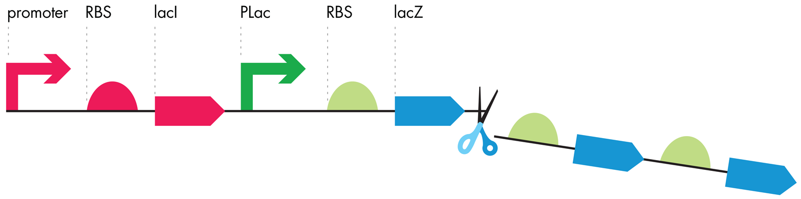
Figure 7-7. Modification of the lac operon. Genetic constructs, such as the ones that are studied in the iTune Device activity, have the second and third RBS-ORF pairs removed. The resulting gene expression unit bears a single promoter-RBS-ORF.

Experimental Question

In the BioBuilder iTune Device lab, you will measure the activity of the lacZ gene product, β-gal, to assess the performance of different promoter and RBS combinations. The promoter and RBS parts have been characterized as “weak,” “medium,” or “strong,” based on their alignment to concensus sequences for such parts. How they will work in combination, though, can depend on culture media, strain background, and techniques for assessing them. If you have the time or interest, you might make these measurements in different bacterial strains, in strains at different stages of growth, or with additional DNA circuits in the living system. Any of these factors might alter how these simple promoter:RBS:lacZ circuits work in the cell.

What might you predict about the activity of these circuits in advance of running the lab to measure them? Table 7-2 can help organize your “guestimates” as well as reveal any biases in your thinking and gaps in your understanding. If we arbitrarily guess that the combination of a weak promoter and a weak RBS will give rise to 10 units, and the strong/strong combination will give rise to 1,000 units, how can we estimate everything in between? The starting values in the chart are theoretical and may not reflect the numbers you get for these circuits when you run this experiment. The point is to ask what it will take to make a good prediction.

In BioBuilder’s iTunes lab activity, β-gal activity is measured because it is an indirect but good reflection of the performance of each circuit. β-gal activity is measured using a substrate called ONPG, a colorless compound that is chemically similar to lactose. β-gal cleaves ONPG just as it would normally cleave lactose. The products of the reaction with ONPG are a yellow compound, o-nitrophenol, and a colorless product, galactose. The yellow compound provides a visible signal, the intensity of which you can use to calculate the amount of β-gal expressed by the different circuits.

To compare data collected by different laboratory groups, you will use a “reference” promoter:RBS:lacZ sequence. This reference is known to generate some intermediate amount of enzyme, so you can use it to calibrate all the other measurements you make. For example, if you measure the reference standard to have 1,000 units of activity and another team measures the same reference to have 500 units, some variation in technique or in the calculation of units might account for the difference. All of your measurements and their measurements, though, should be off by this same two-fold difference, so the data can be compared after that difference is taken into account.

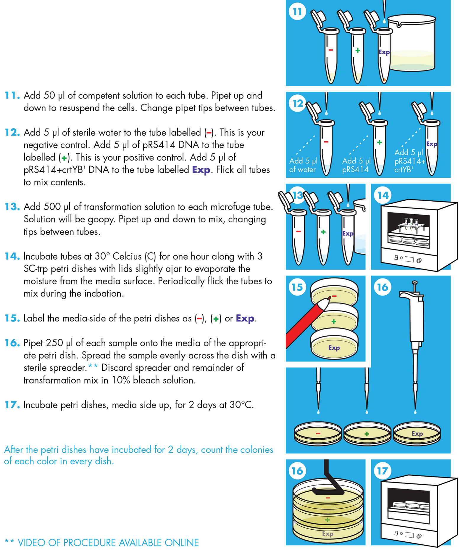
You can consider a reference as a specific type of positive control. We expect the reference sample to produce β-gal and thus the yellow color associated with substrate cleavage. Because everyone doing this experiment will use the same strain as a positive control, to ensure that some enzyme is being detected by the assay, we can also use it as a reference for the exact amount of enzyme being made. For this lab, we have not included a specific strain to use as a negative control. A negative control would not be expected to produce enzyme. Depending on what you want to control for, you could imagine using a strain with no lacZ gene as a negative control or using the reference strain in the absence of the inducer molecule, IPTG. Our experimental question, however, focuses on comparing designs against a reference, and we are less concerned whether the circuits are ON only in the presence of IPTG. We decided a reference strain provides a sufficient level of experimental control to address our question: which combination of promoter+RBS results in the greatest production of β-gal?

Getting Started

There are a total of 10 strains for testing in BioBuilder’s iTune Device activity (Table 7-3). For each of the 10 strains, you will grow a liquid media culture overnight, consisting of LB (growth media), ampicillin to select for the plasmid carrying the promoter:RBS:lacZ construct, and IPTG to relieve inhibition of the lacZ gene.

You will begin the experiment by measuring the cell density of each overnight liquid culture, either using a spectrophotometer to measure the OD600 or using the MacFarland turbidity scale. If you are using a spectrophotometer, the machine measures how much light is scattered by the bacterial sample. Its optical density in 600 nm light (abbreviated “OD600”) is a unitless number that reflects the density of the bacterial culture. Using the MacFarland turbidity samples, which you can convert to OD600 measurements according to Table 7-4, you can carry out this measurement more approximately and with your eyes rather than a machine.

You will then mix a known small amount of each culture—called an aliquot—with detergent, which releases the enzymes from inside the cells into the buffer solution. The buffer keeps the β-gal enzyme stable enough to react with ONPG. You can use the formula that follows to calculate how many cells are in each reaction by measuring the volume of cell culture added to the reactions (measured in ml), and the OD600, which reflects the density of cells in each culture (measured in cells/ml):

Ultimately, with this calculation you can compare the “per cell” enzyme activity between samples.

After the reaction tubes have been prepared, you will start the reactions by adding ONPG, staggering the additions in precisely timed, 10-second or 15-second intervals. The reactions will start to turn yellow. The intensity of the yellow color that develops in a given amount of time reflects the amount of β-gal enzyme that the cells had made before you lysed them. After a known amount of time has elapsed and the reactions are sufficiently yellow, you will add Na₂CO₃, a quenching solution, to stop the reaction by changing the pH. This quenching solution is added in precisely timed 10-second or 15-second intervals so that each reaction can run for a precisely known amount of time, which later makes it possible for you to calculate the enzyme activity/minute elapsed. When the reaction has been quenched, the reactions are stable and so the intensity of the yellow color can be measured at your leisure using a spectrophotometer at 420 nm (Abs420) or comparing to color standards shown on the BioBuilder website.

Finally, you can calculate the β-gal activity for each strain using the standard “Miller Unit” for this enzyme. The calculation is performed according to the following formula:

If you are wondering about the difference between an “absorbance” measurement made on the spectrophotometer and an “optical density” measurement made on the spectrophotometer, here is a simple way to distinguish between them. The reading you take on a spectrophotometer is called an absorbance measurement when the amount of light traveling out of the cuvette is diminished from the light that goes in by a pigment or other molecule in the cuvette that absorbs light. The reading you take on a spectrophotometer is a called an optical density when the material in the cuvette scatters rather than absorbs the light, as is the case by the particles or cells you can measure at 600nm of light. Both absorbance and optical density are unitless numbers and therefore can be used in the calculation of Miller Units without any conversion factors.

Advanced preparation

Prepare turbidity standards

MacFarland turbidity standards shown in Table 7-5 offer an alternative way to measure cell density in cases if you are running the protocols without access to a spectrophotometer. This method uses suspensions of a 1% BaCl₂ in 1% H₂SO₄ that are visually similar to suspensions of the density of E. coli as it grows in liquid culture. You can prepare these turbidity standards well in advance of lab. You can make the turbidity standards in any volume, but you should then suspend and aliquot them to small glass tubes with a cap. The size of the tubes and the volume of the standards you put in them doesn’t matter.

To measure the turbidity of the bacterial samples, you can transfer a small sample of the bacteria to a glass tube that is the same size as the ones used for the turbidity standards. The turbidity is determined by identifying which turbidity standard comparably obscures dark markings placed behind the tubes with the standards.

Rule of thumb: use 1 OD600 ~ 1 x 10⁹ cells/ml to convert the turbidity measurements to cell density.

Pre-lab procedures

Day 1: streak out strains from stabs to plates

The bacterial strains for this experiment already carry the plasmid DNA-encoding genetic circuits to be tested. The plasmids also confer resistance to the antibiotic, ampicillin. The bacteria will arrive as a “stab” or “slant,” which is a test tube with a small amount of bacteria on a slanted media:

1. Streak out the bacteria onto a Petri dish using a sterile toothpick or inoculating loop: gather a small amount of bacteria from the stab on the toothpick or loop, and then transfer the cells to a petri dish containing Luria Broth (LB) agar plus 100 μg/ml ampicillin.

2. Repeat with the remaining stab samples, streaking out each onto a different petri dish.

3. Place these petri dishes media side up in a 37°C incubator overnight. If no incubator is available, a room temperature incubation for two nights will usually yield the same result.

Day 2: grow liquid overnights of bacterial strains

To make a starter culture for the experimental section of this lab, a 3 ml liquid culture of each strain is grown in LB+ampicillin at 37°C overnight. The final concentration of ampicillin in the tubes should be 100 μg/ml, and the final concentration of IPTG in the tubes should be 1mM. A 3 ml starter culture is enough for the protocols that follow. Using a sterile inoculating loop or toothpick or pipet tip, transfer a bacterial colony from one of the petri dishes to a large sterile culture tube containing 3 ml of LB, 3 μl of ampicillin, and 30 μL IPTG. This volume is more than enough for each strain that each student or team of students must grow:

1. Repeat for each strain you will inoculate.

2. Place the culture tubes in the roller wheel in the incubator at 37°C overnight. Be sure to balance the tubes across from each other to minimize stress on the roller wheel.

If there is no roller wheel or incubator available, you can increase the volume for each starter culture to 10 ml LB+amp+IPTG, and you can grow the samples in small Erlenmeyer flasks with a stir bar at room temperature. You should grow them this way for at least 24 hours to reach saturation.

Lab Protocol

With this assay you will determine the amount of β-gal activity produced by each design. You should try to perform replicate assays of each strain and then pool your class data to gain some confidence in the values you measure.

Data collection: turbidity and color using a spectrophotometer

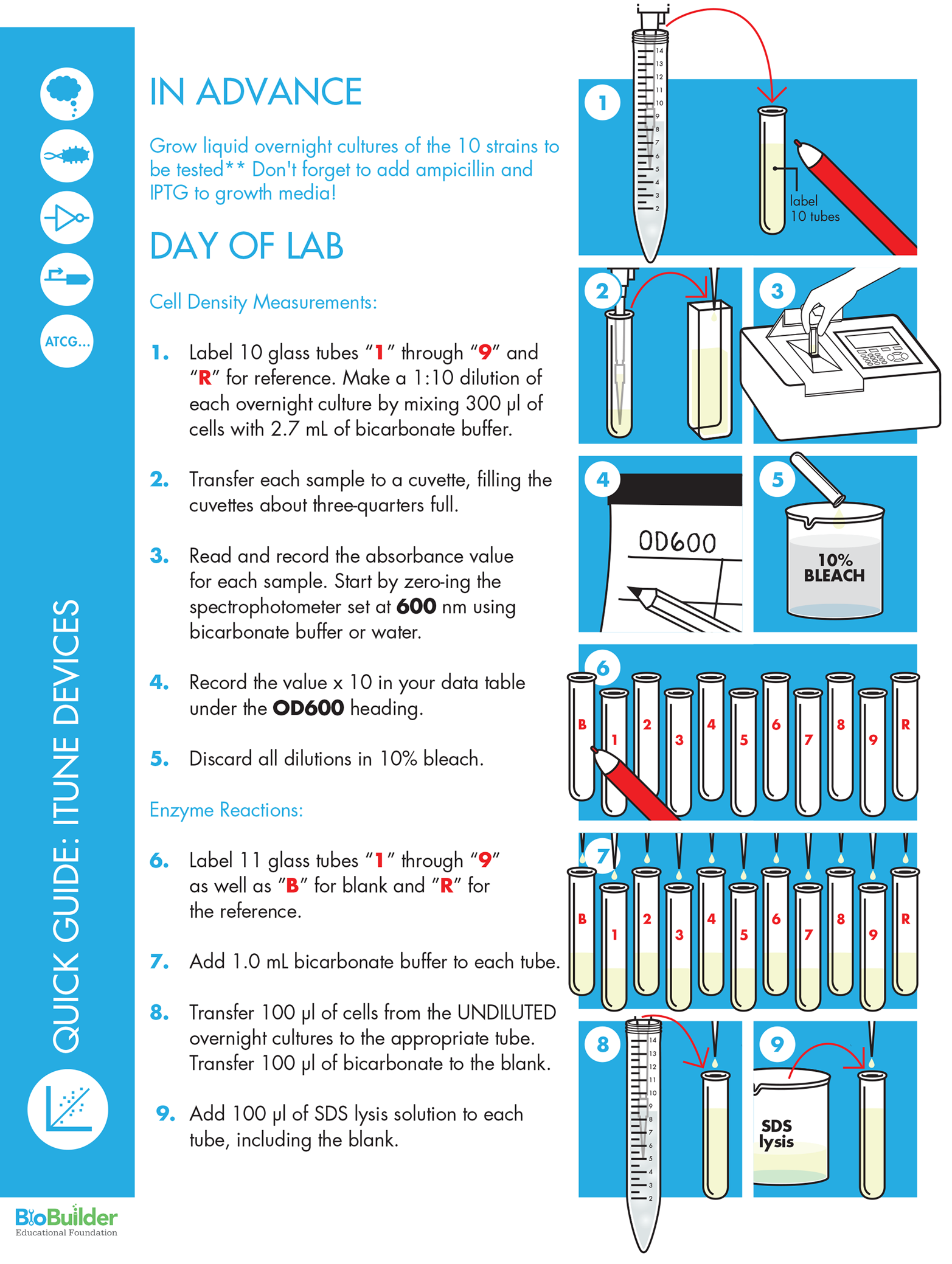
1. Make 3.0 ml of a 1:10 dilution (300 μL of cells in 2.7 ml of bicarbonate buffer) of each overnight culture.

2. If your spectrophotometer uses glass spectrophotometer tubes, you can proceed to the next step. Or, you can transfer the diluted cell mixture to an appropriate cuvette, filling it about three-quarters full.

3. Measure the absorbance at 600 nm (OD600) of this dilution. Record the value X 10 in a data table. This is the density of the undiluted cells. If you do not have a spectrophotometer and are using turbidity standards instead, compare the culture with the MacFarland turbidity standards and use Table 7-4 to convert to OD600.

4. Repeat this data collection with all bacterial samples.

5. You can now dispose of these dilutions and tubes in 10% bleach solution.

6. Add 1.0 ml of bicarbonate buffer to 11 test tubes labeled B (blank), R (reference), and 1 through 9 (the samples). These are the reaction tubes.

7. Add 100 μl of the overnight cultures (undiluted) to each tube. Add 100 μl of LB to tube B, to serve as your blank.

8. Lyse the cells by adding 100 μl of dilute dish soap to each tube.

9. Vortex the tubes for 10 seconds each. You should time this step precisely because you want the replicates to be treated as identically as possible.

10.Start the reactions by adding 100 μl of ONPG solution to the first tube. Simultaneously start a timer or stopwatch to coincide with when you start this first reaction. Wait 15 seconds then add 100 μl of ONPG solution to the next tube. Repeat for all tubes, adding ONPG at 15-second intervals, including the blank.

11.After 10 minutes, stop the reactions by adding 1 ml of the soda ash solution to the first tube. Wait until the timer reads 10 minutes, 15 seconds, then quench the next reaction. Repeat for all tubes, adding soda ash solution at 15-second intervals, including the blank. The reactions are now stable and can be set aside to read another day.

12.If your spectrophotometer uses glass spectrophotometer tubes, you can skip to the next step. If not, you will need to transfer some of the reaction mixture from the reaction tubes to a cuvette, filling it about three-quarters full.

13.Read the absorbance of each sample tube at 420 nm (OD 420). These values reflect the amount of yellow color in each tube. If you do not have a spectrophotometer and are comparing the color to paint chips instead, follow the instructions on the BioBuilder website.

14.Calculate the β-galactosidase activity in each sample according to the formula presented earlier.