BioBuilder: Synthetic Biology in the Lab (2015)

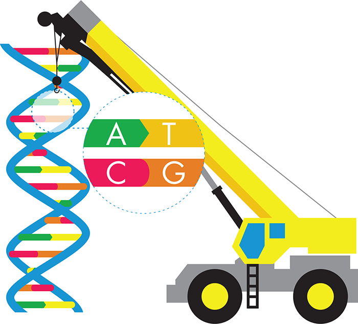
The tools that are available to you for building often define engineering outcomes. For example, new construction equipment like cranes made it possible to build skyscrapers, and ever-improving transistors have made our computers run faster and faster. In this chapter we consider a key tool for synthetic biology, namely the engineering of DNA. If we want our fluency in writing genetic code to match our fluency in other programming languages, there must be ways to write, compile, and debug DNA code with ease. In this chapter, we consider how the engineering technique of standardization can help meet that goal and how the current tools for DNA engineering work and fit in that context.

Framing the Discussion

Easy does it. Take it easy. Easy as pie.

Cultural idioms that equate “easy” with “happy” are everywhere. We seem to yearn for a life with fewer challenges, and for a time when things work effortlessly. Who wouldn’t want that? It turns out, however, that it’s not simple to make things easy. As an example, think about the ubiquitous automatic dishwasher appliance. At last count dishwashers are found in around 85 percent of American homes, despite the fact that we can accomplish the same task with just our hands, some hot water, and a sponge. Clearly the majority of homeowners think it’s easier to throw the forks into a machine than to clean them by hand.

Putting dishwashers into so many homes, however, took more than 150 years of invention. Dishwashers started as wooden boxes with a hand-crank to spin a rack of dishes through splashing water. The first reliable timesaving dishwasher was the patented invention of Josephine Cochrane who was fed up with the damage her fine china endured from hand washing. The appliances became widely available thanks to the founding of the KitchenAid company (by the same woman who patented the invention) and to multiple upgrades in modern plumbing. It could even be argued that dishwashing has been made easy thanks to the invention of water heaters, dish soaps, and weekly allowances that could be offered to kids for emptying the dishes from the dishwasher. What’s clear from this example is that making things easier takes a lot of hard work, and often takes a long time.

The hard work involved in making things easy is relevant here because many synthetic biologists want to make biology easier to engineer. Anyone who has been in a biology research lab will tell you that the field has a long way to go to meet this aim. It’s challenging to make biology behave the way we intend. In living cells, variations abound and we have good but not full understanding of how cells work. Consequently, experiments that look easy often take much longer to accomplish than expected, if they can be successfully completed at all. Engineers are frustrated by the delays and unpredictability of these efforts, and they are urging synthetic biology to make long-term investments into foundational construction tools, common programming languages, and fabrication centers. They argue that we couldn’t have built sophisticated structures such as the Empire State Building without cranes that lift enormously heavy objects, blueprints that builders could follow, and steel mills to provide the needed building materials, so how can we build sophisticated biology without similar resources for design and construction of living cells?

The tension that becomes apparent is the one between the time and effort it takes to make improvements in the engineering tools and the eagerness everyone feels to get a given job done. The dishwasher example we considered earlier illustrates an older case of this same tension. It is reported that Josephine Cochrane was disgusted at how long it was taking anyone to make a mechanical working version of the machine so she invented it herself in 1866. However the cost of her first dishwashers was high, making them suitable only for commercial venues such as restaurants and hotels. It took more than 50 years of cost reductions and incremental engineering improvements for the dishwasher to become a household item.

In this chapter, we explore a foundational element of synthetic biology that must improve if the engineering of biology is ever to become easier: DNA engineering. We will focus on standardization as one approach to facilitate the process, drawing inspiration from historical examples in more robust engineering disciplines. We apply these ideas about standardization to DNA engineering by looking at cloning and Polymerase Chain Reaction (PCR) techniques that are now more than a generation old, and then we turn our focus to some of the more current techniques for assembling DNA sequences.

Standardization of Parts and Measurements

Standards, such as the shape and voltage of an electrical socket (as shown in Figure 3-1) and the standard measure of a cup or a gram, make engineering—and life—easier by bringing consistency and a common vocabulary for describing things. By agreeing to certain standards as we build or measure, we can feel confident that parts will “match up” when we put them together. In the absence of standards, we run into frustrating inconsistencies—like when we’ve brought the wrong charger for a phone or laptop.

Figure 3-1. Variations in electrical socket standards across the world. Electrical socket standards vary across the world, requiring unique plugs in Australia (left), Italy (center), and the United States (right).

What Is Standardization?

Standardization is a key attribute of mature engineering disciplines because it makes it possible for engineers to more quickly implement exciting, innovative, and useful solutions. For example, consider the manufacturing assembly lines that arose during the Industrial Revolution. Before that time, most products were hand crafted, often by a single person who painstakingly made all the individual parts and put them together. This process changed and manufacturing was revolutionized by the availability of standard and interchangeable parts. Individual pieces could be produced by machine in one factory and then assembled into a variety of products elsewhere. Suddenly a lever made in one location could be used in the manufacture of a clock, a sewing machine, or a train car, thereby increasing the efficiency of manufacturing and accelerating the engineering design cycle. Without question, the availability of standardized parts has allowed engineers to more rapidly prototype new ideas.

Commonly standardized features include the size, shape, material properties, and behavior of components. These aspects can be important for proper assembly of parts, as illustrated by the clever design of LEGO blocks. LEGO pieces snap together easily because they all have bumps and holes of a certain size and spacing. The bumps on the top of any LEGO piece fit into the holes on the bottom of any other LEGO piece, and the pieces are all made of the same hard plastic so they can be interchanged and used to build many things.

Electrical sockets around the world provide an interesting counterpoint to assembly standards for parts. In this case, “assembly” means plugging an appliance into a socket. Over time, countries across the world have developed different sizes, shapes, and voltages for their electrical sockets. Consequently appliances designed for use in the United States can’t be used directly in other countries because the plug simply won’t fit into the socket. Based on this discussion, you might be thinking, “Hey, wait a second, if there are all types of electrical sockets around the world, these things must not be standardized at all!” The truth is that standardization doesn’t necessarily mean agreement on one single standard; another person could, for example, make LEGO-like bricks with different size or spacing for the bumps and holes. Nonetheless, each country—or LEGO-like block manufacturer—must have its own internally consistent standard, but all parts in existence do not need to be universally interchangeable. The drawback to variability is the parts are no longer perfectly interchangeable.

In practice, therefore, engineers agree upon a finite number of standards to use, which can work well as long as they can be interconverted and that it’s clear which standard unit is being used for a given project. Length measurements provide an excellent example of both the importance of standards and the existence of competing standards, as we will discuss in the next section.

Competing Standards

Standards can (and do!) come from anywhere. For example, the “foot” measure (Figure 3-2) that’s used primarily in the United States was originally based on the approximate length of a human foot. Of course, foot length varies greatly between different people, so in its original form, this “length of my foot” standard might have been useful for an individual, a builder for example, working alone to build a house. However, if this builder needed to get material from a carpenter, the builder was in trouble if his feet and those of the carpenter’s feet weren’t the same size. The needed 16-foot-long boards might be too long or too short depending on who had the bigger feet. Of course, now we have a standardized foot measure to eliminate such inconsistency.

Figure 3-2. Examples of competing standards. Some examples of competing standards we are familiar with are English versus metric length measurements (left), .tiff versus .jpg image files (center), and alternating current (AC) versus direct current (DC) (right).

An alternative distance standard, the meter, was originally defined as one ten-millionth of the distance between the equator and the North Pole. This distance does not vary from person to person, but it is difficult to measure independently. If the builder working on his house measured materials in meters rather than measuring them with his feet, he could not directly measure the fractional distance from the equator to the North Pole, and so he would need a meter stick to estimate all the lengths, as would the carpenter.

The foot and the meter are alternative units for length, and they provide an example of competing standards and how each alternative has strengths and weaknesses. The foot is more immediately useful, whereas the meter is more standard. There is not a “right” or “wrong” for any given standard, just one that might be more or less appropriate for specific applications. In the case of the builder who needs boards from the carpenter, what’s important is that they both use the same unit, or else the boards that were intended to be 16 feet in length could arrive measuring 16 meters. And now that both the foot and the meter are standardized, engineers can also convert between the two measures if needed, so the existence of the two standards is workable.

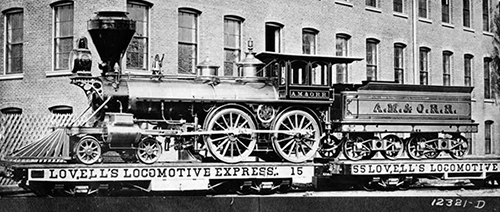
Competing standards, even interconvertable ones, can lead to some absurd workarounds. For example, in 1873, Mason Machine Works in Taunton, Massachusetts, manufactured a beautiful new train engine for the Atlantic, Mississippi & Ohio Railroad. But because the gauge of the rail was different in Massachusetts, where the train was made, and in Ohio, where it was being delivered, the train couldn’t ride on the tracks in Massachusetts and had to be carried to its destination on a flat car.

This example illustrates the clear benefits of a standard unit, but in practice, developing and adhering to a single standard can prove difficult for any field. In addition to the competing English and metric measurement systems, other historical examples include Betamax versus VHS for videos and alternating current versus direct current for electricity. Perhaps various stakeholders have different goals or priorities, and these preferences cause them to promote one standard over another. Even a standard that is superior to another can present technological, practical, and psychological barriers if promoted as a replacement.

How Standards Are Established

Part of the reason that so many competing standards exist across all fields is that standards can arise in an ad hoc way. An individual researcher or engineer might develop a measurement or manufacturing practice that suits a particular need. Others might then see that unit as useful and adopt it, perhaps making slight modifications so it better suits their own purposes. This type of organic standards development can be messy as researchers adjust the unit in different ways for their own purposes, creating slight variations within the emerging standard, but it can also provide an excellent opportunity for experimentation and optimization. The gradual consensus-building around such an informally developed “pseudostandard” can save time and money, too, especially in rapidly changing fields that are prone to develop in unexpected directions, making the ultimate required standards unknowable at the outset.

Dr. Jason Kelly, a synthetic biologist working on foundational advances for the field, cited the laying of the first trans-Atlantic cable in 1858 as an instructive study in ad hoc standard development. Because the trans-Atlantic cable had to operate under water, engineers were confronted with measurement and repair challenges that they’d never faced when working with the land telegraphy lines in the 1840s. If the landlines didn’t work, they could be visually inspected, measured, and then adjusted into proper operation. A different plan was needed for the repair of the undersea cables because there was no easy way to visually examine them. Instead, the engineers went back to basics. Manufacturers of the cable’s copper wires could measure their electrical characteristics using various types of batteries to produce a standard voltage and calibrated galvinometers to record current. The measurements revealed that the resistance of each cable varied considerably from manufacturer to manufacturer, which was not really surprising given that the copper in the cables was only 50 percent pure at best. Nevertheless, precise measurements of the conductive properties allowed even nonuniform units of copper wires to be assembled into cables that could operate for more than 2,000 nautical miles and under as much as 12,000 feet of ocean water. The 1858 cable was successfully laid, and the time it took for Queen Victoria and President James Buchanan to exchange messages between England and the United States dropped from days to hours.

The telegraphed messages ended, however, after just three weeks when the insulation of the undersea cable failed, and the cable had to be abandoned as unrepairable. However, as the technology improved in the next few years, faults on subsequent cables could be traced from the shore ends of the cable. To locate the fault, even roughly, cable manufacturers relied on their precisely recorded resistivity measurements, and then repair ships were dispatched to the approximate point where the circuit failed. Locating the fault in the telegraph line did not rely on a resistivity standard but rather on the anticipated behavior of the nonuniform cable.

By the late 1860s, a uniform standard for resistance was recommended to better compare the data collected by each cable manufacturer. The British Association for the Advancement of Science produced a new physical reference standard to define this new standard. The reference object was a coil of platinum alloy in a brass enclosure, which they declared produced 1 ohm of resistance. The definition was somewhat arbitrary—there is nothing magical about the exact amount of resistance that is a single ohm—but it provided the necessary benchmark. This reference standard was easy to reproduce, so it could be broadly distributed to the various cable manufacturers, along with instructions on how to measure resistance with it, as is depicted in Figure 3-3. The reference standard made it easier for many manufacturers to measure their cable’s electrical properties, and it allowed the measurements to be compared between manufacturers. The initial reference ohm wasn’t a perfect standard and it has been adjusted over time. Even so, the early effort at standardization proved to be useful for the specific application of undersea telegraph lines, and it kick-started the development of the ohm standard.

The lessons from this example are particularly relevant for synthetic biology, which itself is in the early days of standardization. For many years biology labs around the world have been constructing genetic circuits from DNA snippets using a variety of techniques, some of which are described in the next section. Synthetic biology, though, emphasizes scalable assembly of genetic circuits, which requires standardizing the assembly of DNA. The next section also describes some early ideas and efforts that standardize the way DNA parts are put together.

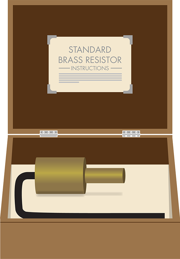
Figure 3-3. The reference object for defining the standard ohm. This image resembles the physical reference standard used to define the ohm as a measure of resistance. It included a metal object for making resistance measurements and instructions for its use.

DNA Engineering in Practice

Having introduced the role standardization plays in other engineering arenas, we will now explore how it applies to synthetic biology and the physical assembly of the major building blocks in synthetic biology: DNA.

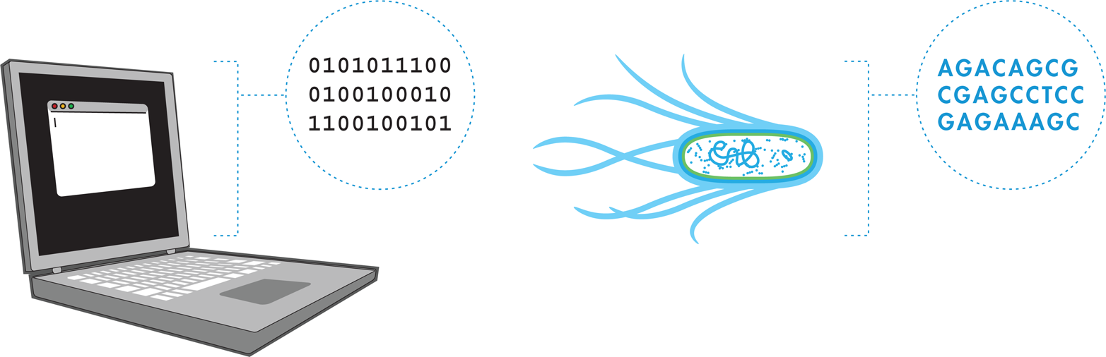
You might be thinking to yourself, “Biological function requires so many important molecules, like proteins, lipids, and both DNA and RNA—don’t we need more than DNA to engineer biology?” You are right to note that DNA itself is an inert molecule and only one of the key players in a cell’s function, but because information generally flows from DNA to RNA to protein (a paradigm known as the central dogma), any changes to an organism’s DNA will affect all downstream functions. It is the DNA-encoded products such as the cell’s enzymes and structural molecules that are responsible for executing the biochemical functions that allow the cell to function. At the end of the day, it is these functions that must be manipulated, which is accomplished by engineering DNA. In other words, part of the power and beauty of building biological systems is that cells can change their molecular composition based solely on the DNA sequences they contain. In this way, they behave somewhat like computers reading software, except that instead of interpreting zeros and ones, cells read instructions that appear in the language of DNA.

DNA is a big molecule—more specifically, it is a polymer of four types of nucleotide building blocks attached head-to-tail into strands that can be millions of nucleotides long. DNA follows the same chemical rules that other molecules follow, so synthetic biologists can engineer DNA from scratch by forming bonds between the nucleotide monomers. In addition, synthetic biologists can break and rebuild bonds between bases from naturally occurring DNA that’s been extracted from biological systems. Most commonly, synthetic biologists use a combination of these two approaches to assemble “synthetic” and naturally occurring DNA pieces into new and desired genetic circuits. To do this, engineers have found clever ways to co-opt naturally occurring enzymes responsible for similar processes in the cell to perform the DNA engineering reactions in a test tube in a process referred to as molecular cloning (see the sidebar on “Origins of Cloning Enzymes”).

The end product of DNA assembly is called recombinant DNA (rDNA). rDNA refers to DNA made in the laboratory with the techniques of molecular cloning. The resulting DNA can be a combination of sequences that might or might not appear in nature. Developed decades before the modern field of synthetic biology, rDNA is part of the traditional molecular biology toolkit described in the Fundamentals of Synthetic Biology chapter. In the following sections, we describe some common principles among DNA manipulation approaches. We then explore three specific methods that employ differing levels of standardization, each of which has its own advantages and drawbacks.

DNA Assembly Basics

DNA assembly requires a few basic components and tools:

§ Plenty of DNA, coding for the specific functions needed

§ A way to precisely combine DNA pieces

§ A way to introduce these engineered DNA components in the target organism

The methods available to manipulate DNA are inefficient, so in general DNA engineers begin with as much DNA as possible and then select for the relatively rare DNA combination that contains all the desired DNA components. There are a few different ways to produce lots of initial DNA, including PCR, plasmid preparations, and synthesis. These processes, which are discussed in more detail as we proceed, can be used alone or in combination to produce a wide array of recombinant DNA.

rDNA is often introduced into cells as small, circular pieces of DNA called plasmids (see Figure 3-4) via a process called transformation. You can read more about the transformation process in the What a Colorful World chapter. An alternative to plasmid-based approaches for DNA engineering is the direct editing of an organism’s genome, which is possible but which we will not address here. Simple plasmid preparation protocols can provide the needed amount of DNA as starting material for further experiments. There are many commercially available plasmids that we can manipulate with restriction enzymes (see the sidebar on “Origins of Cloning Enzymes”). Minimally, plasmids encode a selectable marker, often one that confers resistance to a drug, and a multiple cloning site, which is a region containing many restriction sites where we can easily insert or remove genes. Such a minimal plasmid might be purified to serve as a blank canvas or “backbone” into which an engineer can then build new genes. Alternatively, a plasmid might already include a gene of interest; in such cases, the plasmid is purified in order to extract that gene from the plasmid with a few subsequent steps. In either case, plasmid preparation methods take advantage of the cell’s natural ability to replicate, making many copies of its DNA with minimal human effort or intervention. Because plasmid DNA is often easier to manipulate than genomic DNA, rDNA is generally maintained in plasmid form throughout the cloning process.

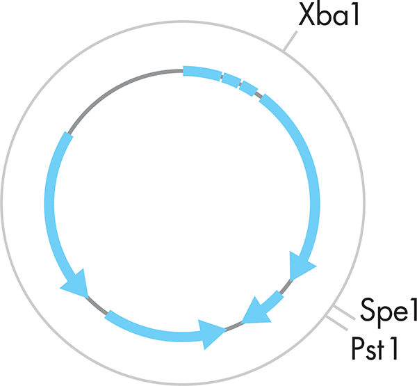
Figure 3-4. A standard plasmid representation. The gray circle represents the plasmid. The blue arrows represent the functional portions of the plasmid, with the arrows representing the direction of transcription required for that component. XbaI, SpeI, and PstI mark sites that would be cut by the corresponding restriction enzyme.

PCR (Figure 3-5) is another common approach to producing the necessary DNA for assemblies. You can read more about PCR in the Fundamentals of Synthetic Biology chapter. Briefly, using PCR, engineers can generate many copies of a specific DNA sequence, usually up to a few thousand nucleotides long, in a linear form, starting with only a very few copies of it. Beyond the needed DNA starting material, also called template DNA, PCR requirespriming oligomers, sometimes called “primers” and sometimes called “oligos,” which are short polymers of DNA up to about 50 nucleotides in length. To carry out PCR, template DNA, priming oligomers, enzymes, and buffers are placed in a machine to cycle through different temperatures. The DNA produced by PCR can later be inserted into a plasmid, allowing copies of the DNA sequence to be isolated by simple plasmid preparations as previously described. In addition, the DNA produced by PCR can be engineered to include some useful modifications. For example, it can be appended with short sequences such as restriction sites by incorporating the desired modifications into the priming oligomers.

Figure 3-5. Polymerase chain reaction. The blue bars represent the region of DNA sequence to be amplified, and the black arrows represent the priming oligomers that define the edges of that sequence.

Chemical DNA synthesis (Figure 3-6) is one more way to generate DNA. Nucleotides are added one by one in a test tube to a growing chain of single-stranded DNA. There are several advantages to direct chemical synthesis of DNA, however. For one, the nucleotides are attached to one another chemically, without the need for any template DNA. Thus, the desired gene can be produced solely from the digital information about the desired sequence and does not have to previously exist in nature. Another advantage of chemical DNA synthesis is that the construction of the product is outsourced, which frees up a researcher to focus on other experiments. At this point, though, chemical synthesis is most routinely used to make priming oligomers for PCR. By itself, this approach to making DNA is constrained by the cost associated with the synthesis, the time it can take to generate the product, and some persistent technical limitations on the synthesis of very long sequences. But, hybrid approaches that combine chemical synthesis of short DNA sequences with PCR-based assembly methods are becoming increasingly commonplace as a means for acquiring genes, both natural and synthetic.

Plasmid preparations, PCR, and chemical synthesis are all recognized methods to generate starting materials to assemble into rDNA. To “cut” and “paste” the DNA starting materials, restriction enzymes are often used. These endonucleases cut double-stranded DNA only when they recognize a particular DNA sequence, called a restriction site. There are hundreds of kinds of restriction enzymes, each of which acts like a pair of scissors, recognizing and cutting their specific DNA sequence and leaving some of the DNA bases either flush (“blunt ends”) or unpaired (“sticky ends”), as shown in Figure 3-7, depending on the enzyme. If different pieces of DNA are cut with the same restriction enzyme, the resulting ends will be complementary, and the bits of DNA can connect to each other. If multiple enzymes are used, multiple “sticky” overhangs can attach the cut DNA segments to each other. After they’re connected, the final step in rDNA assembly is to “paste” the pieces, usually using an enzyme, DNA ligase. Ligase seals the cuts in the DNA where the restriction enzymes broke the bond in the DNA’s phosphodiester backbone. Restriction enzymes and ligases are convenient tools for molecular and synthetic biologists, but if you’re curious why they exist in nature, the sidebar that follows explains the origins of cloning enzymes.

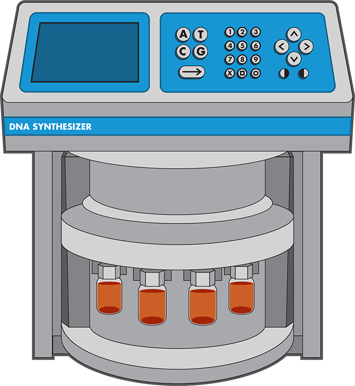
Figure 3-6. A DNA synthesizer. The four orange vials represent the reagents, one for each DNA base to be assembled into a DNA chain. The computerized interface at the top allows the engineer to input their desired sequence.

Figure 3-7. Recombinant DNA. The pairs of black and blue bars represent double-stranded DNA, color coded to show where it has been cut with restriction enzymes to leave complementary “sticky ends” (left) or “blunt” ends (right) that can reconnect as shown.

ORIGINS OF CLONING ENZYMES

The enzymes used for cloning DNA are sourced from existing organisms. Cells need DNA polymerase, for instance, to relicate their genomres prior to cell division. Restriction enzymes and ligases also play important roles in cell survival and proliferation:

Restriction enzymes

Bacterial cells use restriction enzymes to defend themselves from invasion by foreign DNA (for example, viruses). These enzymes evolved to cut specific DNA sequences, collectively called restriction sites. Restriction sites are typically four to six base-pairs long. When a virus injects its DNA into the host cell, the restriction enzymes of that cell snip the DNA into many pieces, preventing its insertion into the host’s genome and inhibiting infection. Any given species of bacteria produces only one or a few types of restriction enzymes because as the number of restriction enzymes in a cell increases, it becomes ever more likely that restriction sites will also exist in the host’s own genome. Having a genomic copy of a restriction site could prove destructive because the restriction enzyme that recognizes it could destroy a cell’s own genome. The available collection of nearly 600 commercial restriction enzymes comes from hundreds of different organisms, and they recognize restriction sites that are absent or modified in their host’s genome to prevent the enzymes from chopping the cell’s DNA to bits.

Ligases

Cells normally use DNA ligases for DNA replication and repair. During replication, one of the DNA strands, called the lagging strand, is synthesized in discontinuous segments. DNA ligase is used to connect these fragments to produce a single continuous chain. In addition, ligases reseal nicks in the DNA backbone that are generated when DNA is damaged or when an incorrect nucleotide is excised and replaced by the proofreading mechanism active during DNA replication. Ligases are used in molecular biology to seal the nicks that remain in the DNA backbone when sticky-ends of DNA base pair.

Applying the Basics of DNA Assembly

Thus far, we have focused on commonplace ways that DNA is prepared and then introduced into a cell. Next, we explore how different pieces of DNA can be specifically and precisely combined. To illustrate, we describe how different strategies of DNA assembly could be used to make the plasmids, which take center stage in the iTune Device chapter. It is not necessary to have read that chapter to follow along. All you need to know is that the iTunes laboratory investigation tests how much β-galactosidase enzyme is produced when the gene is controlled by regulatory elements of different strengths. Each of the plasmids used in the iTunes experiment include one of three possible promoters and one of three possible ribosome binding sites (RBS) upstream of the enzyme’s coding sequence. The promoters direct transcription of the gene by recruiting RNA polymerase, and the RBSs initiate translation by the ribosome to produce the enzyme (Figure 3-8). All possible combinations of these DNA elements plus one reference plasmid have been assembled previously. Here we examine how they could have been made using traditional cloning techniques (see “Building DNA: traditional molecular cloning”), BioBrick assembly (in “Building DNA: BioBrick assembly”), and Gibson assembly (“Building DNA: Gibson assembly”).

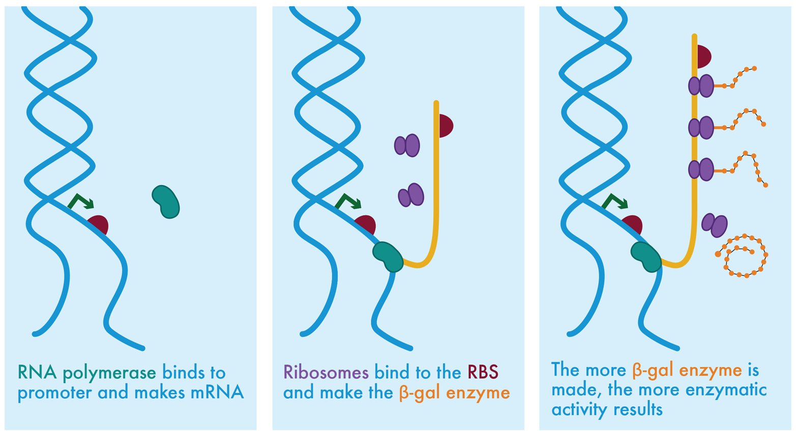
Figure 3-8. Molecular biology’s central dogma. In the leftmost panel, RNA polymerase (green bean shape) is shown near the promoter region of unwound DNA. The promoter region consists of the promoter (green arrow) and the RBS (maroon semicircle). In the center panel, the RNA polymerase has bound to the promoter and started to transcribe the mRNA (shown as an orange strip). Ribosomes, shown as purple shapes, are collecting near the ribosome binding site on the mRNA. Translation of the mRNA into proteins is shown on the right, with synthesis of the orange protein progressing as each ribosome translates farther along the mRNA.

As you will see, each strategy has its own advantages and disadvantages. Traditional molecular cloning techniques can work reliably but you must developed them on the spot for each new DNA assembly challenge, and thus they require considerable expertise to plan and execute flawlessly. BioBrick assembly represents one of the first attempts to standardize traditional cloning. It has gained wide acceptance by International Genetically Engineered Machines (iGEM) teams because it is compatible with many of the freely available BioBricks in the Registry of Standard Biological Parts. Gibson assembly is a relatively new technique that is compatible with BioBrick parts but does not require them. Gibson assembly, which enables the simultaneous assembly of many pieces of DNA, is considered by many to represent the future of DNA assembly, but as yet it has not achieved the standardization required for a mature engineering method. One day, Gibson assembly, like BioBrick assembly, might become a standardized technique, but as with other new technologies, standardization lags behind innovation.

Building DNA: traditional molecular cloning

The three elements cloned onto the iTunes plasmids are a promoter, an RBS, and the coding sequence for the β-galactosidase enzyme. β-galactosidase is a naturally occurring enzyme encoded by the lacZ gene found in E. coli. Because there is a natural and readily available source for the lacZ gene and because the gene’s sequence is known, PCR is a logical approach for making enough starting lacZ DNA to clone. It’s less obvious how to make enough of the promoter and RBS starting materials. Natural versions of these exist but they can also be invented based on an idea for a new promoter or RBS with particular properties. In addition, promoter sequences are short, around 35 bases, and the RBSs are even shorter. The most common approach for generating such short pieces of starting DNA is to chemically synthesize DNA oligomers that can later be combined in a test tube to generate the desired double-stranded DNA sequence. Often times, it’s also sensible to include restriction sites at either end of the synthesized sequence, allowing the sequence to be manipulated and cloned. Commercial DNA synthesis is reasonably inexpensive, with companies offering their services for pennies a base. They also often send enough DNA so that it can be used as starting material for the first few cloning steps.

When the DNA starting materials are in hand, there are a number of next steps to clone the promoter, RBS, and lacZ gene into a plasmid using traditional molecular cloning techniques (see Figure 3-9). Generally speaking, you need a start-to-finish strategy because usually only one piece of DNA is inserted into a plasmid at a time. For example, to make the iTunes plasmids, it might have been sensible to cut the starting plasmid and the lacZ PCR product with two restriction enzymes: we’ll call these enzymes “C” and “D.” Ideally, enzymes C and D will leave sticky ends to the pieces so the lacZ and plasmid DNA segments can bind to each other in a predictable way. The two DNA pieces could then be ligated, transformed into E. coli, and selected for growth on a drug-containing media. You could then purify successful clones of the new “lacZ+plasmid” DNA from the cells by plasmid preparation and carry them on to the next step, which is to add the RBS. You could carry out this DNA assembly by using restriction enzymes “B” and “C,” which might leave sticky ends that align these pieces of DNA properly. Again, you could ligate the pieces, transform them, and then select colonies for subsequent growth to produce many copies of the desired plasmid. After the “RBS+lacZ+plasmid” DNA is verified as correct by sequencing the DNA or verifying its pattern with restriction enzymes, you could finally cut it again, along with the starting promoter DNA material, using restriction enzymes “A” and “B” this time. One more time, the DNA components could be ligated, transformed, selected, and (at last) prepared as the final desired plasmid.

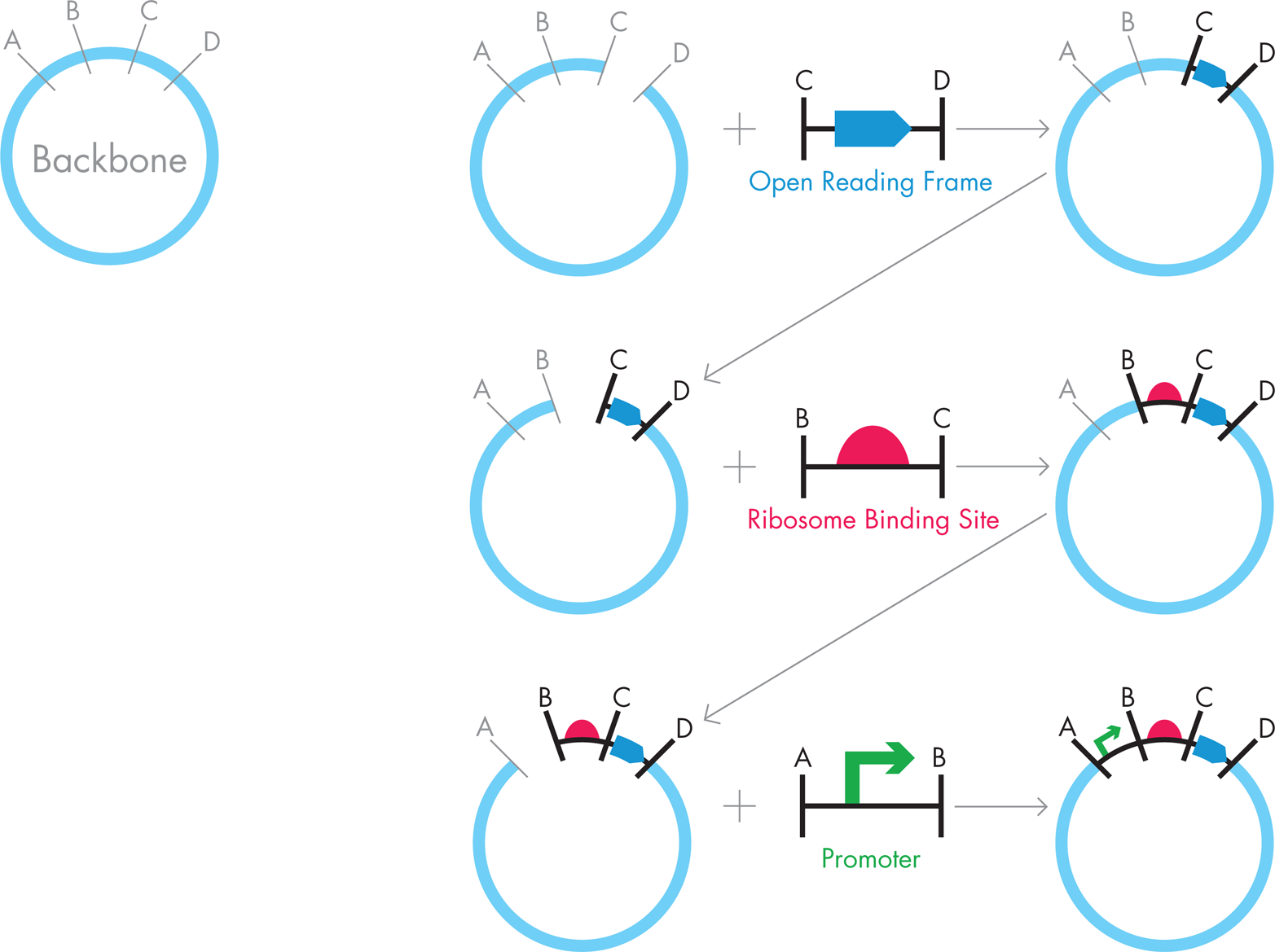
Figure 3-9. Traditional cloning. To make a single iTunes plasmids using traditional cloning, a backbone plasmid could be cut with restriction enzymes “C” and “D,” and PCR could be used to generate the desired DNA flanked with “C” and “D” restriction sites. These fragments, when ligated together, create a new backbone, which would then be cut by enzymes “B” and “C” and combined with the “B” and “C” flanked DNA for the RBS. The resulting backbone would then be cut one more time, this time with enzymes “A” and “B,” and combined with the “A” and “B” flanked DNA for the promoter to assemble the final iTunes plasmid. Between each step, the new backbone plasmids must be transformed into E. coli and grown so that the DNA can be extracted, and verified as correct.

Phew! Several days later, this strategy could yield one of the ten plasmids needed for the iTunes lab as shown in Figure 3-10 (but see the upcoming sidebar “DNA Engineering in Real Life” to learn about some of the ways that this process may not be successful). Happily, you could reuse some of the plasmids that were made as intermediates (for example, the “RBS+lacZ+plasmid”) to aid in the assembly of the other plasmids. By starting the cloning with the lacZ gene, which needs to be in all of the plasmids, you could do many of the subsequent steps in parallel.

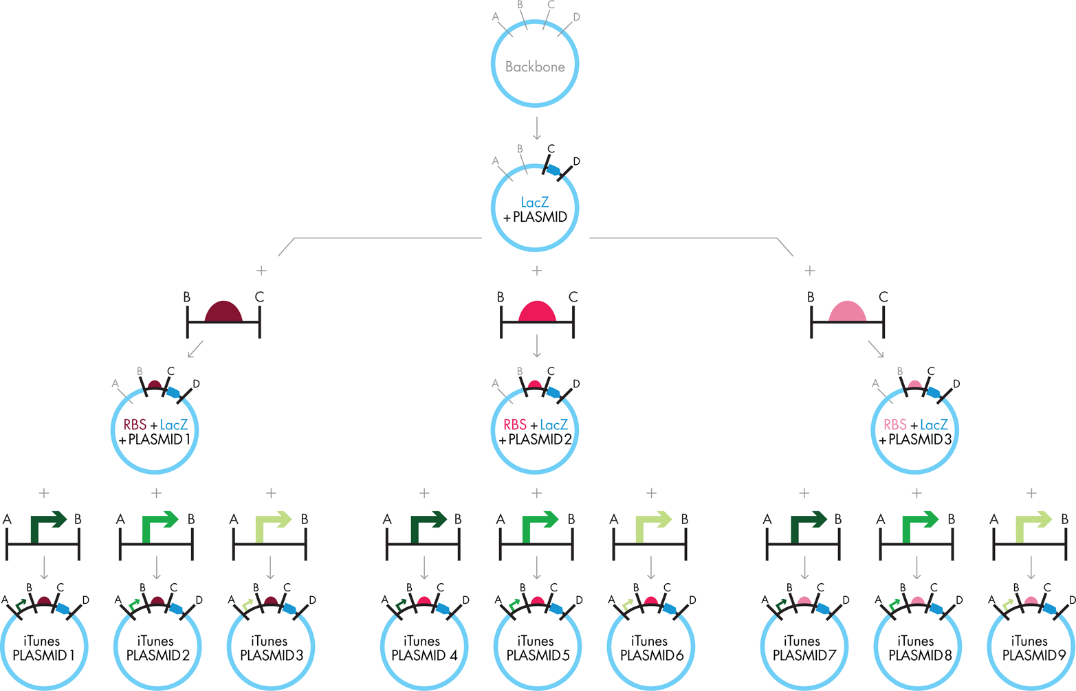
Figure 3-10. Scaling traditional cloning. The traditional cloning approach shown in the Figure 3-9 can be scaled to produce a library of iTunes plasmids by separating the product of the first reaction into three different batches, conducting the second cloning step using a different RBS in each reaction, and then separating each of these product plasmids into three batches for the final step of adding the different promoters. The strategy outlined here works only when none of the needed restrictions sites (“A” “B” “C,” or “D”) exist within the fragments to be cloned.

Overall, using traditional cloning, and assuming all the steps proceed perfectly, it would require at least several days and approximately thirteen digestion/ligation reactions to assemble all of the iTunes plasmids. If you’re thinking there should be a less idiosyncratic and faster way to assemble DNA, you are thinking the way many synthetic biologists do. BioBrick and Gibson Assembly are two methods that arose in part from frustrations with the pace and ad hoc nature of the traditional molecular cloning techniques.

DNA ENGINEERING IN REAL LIFE

Our discussion of traditional molecular cloning can make the process seem cumbersome, but it actually presents the best-case scenario. Cloning in real life can hit many snags, including misbehaving primers, cells with poor transformation efficiency, and inactive enzymes. That’s just lab life—researchers sometimes must spend time troubleshooting and optimizing procedures that, by all appearances, should work but don’t. You might experience this yourself as you carry out some of the BioBuilder labs. There are entire lab manuals dedicated to addressing these types of issues, and it’s not our focus here. Nonetheless, we want to introduce a few of the common pitfalls to give you a better idea of what it means to actually conduct DNA engineering in the lab.

Sequence Editing for Restriction Enzyme Use

Restriction enzymes are a crucial tool for various genetic-engineering approaches. Engineers use them to cut DNA at specific signature sequences so that they can manipulate that part of the sequence, for example by inserting a new piece of DNA. The enzymes’ sequence specificity is crucial for allowing the engineers to implement their design in a controlled, targeted way, but the DNA sequences the engineer is using might need to be altered to make them amenable for use with a specific restriction enzyme. Specifically, the enzyme’s target sequence must not exist anywhere in the sequences other than where the engineer wants it to cut. If the sequence exists somewhere it shouldn’t, the engineer must change it, perhaps using an approach called site-directed mutagenesis, before proceeding with the rest of the cloning. Luckily, the redundancy of the genetic code means that, in most cases, the problematic sequences can be changed without changing the amino acid sequence. For example, if TTC in a DNA sequence is changed to a TTT, the EcoRI recognition site is mutated but the sequence still encodes a phenylalanine.

Troubleshooting and Changing Strategies

Even the most carefully planned cloning protocol can fail, due primarily to the somewhat unpredictable behavior of biological systems. For instance, crucial enzymes, including restriction enzymes, nucleases, and ligases might stop working if they were left out of the freezer for too long. The cells can lose their transformation efficiency, making it essentially impossible for the engineer to even know if the previous cloning steps work. Most of these problems are relatively easy to fix—the researchers can order new enzymes from a company or grow up a new batch of cells—but it takes time, and so the setbacks add up. Other lab problems can be more difficult to solve. Sometimes, certain primers or a specific cloning strategy don’t work for any apparent reason. This can be very frustrating for scientists, who always want to know why things are happening, but usually the best tactic is to simply move on and try a completely new approach, because the traditional cloning toolbox is big enough that there are almost always multiple ways to engineer a certain sequence.

Building DNA: BioBrick assembly

Like traditional molecular cloning, BioBrick assembly is based on a strategy that uses restriction enzymes and ligases to piece together segments of DNA. However, because all the DNA segments come as standardized BioBrick parts, some steps are streamlined and other steps are skipped entirely. BioBrick parts are defined as DNA sequences that provide a specific biological function. Commonly, promoters, RBSs, and open reading frames (ORFs) each are defined as simple “parts.” Each BioBrick part has a unique identifying part number. For example the lacZ sequence on the iTunes plasmids is part BBa_E0051, with “BBa” standing for “BioBrick series a” and E0051 indicating the catalog number for the part’s unique information on the Registry of Standard Biological Parts. The promoter parts and RBS parts that are on the iTunes plasmids also have unique identifying part numbers so anyone with an Internet connection can look up information about their sequence and their behavior.

As originally described by Dr. Tom Knight at MIT, each standardized BioBrick part is sandwiched between a uniform “prefix” sequence containing the restriction sites for EcoRI and XbaI, and a uniform “suffix” sequence containing the restriction sites for SpeI and PstI, as illustrated in Figure 3-11. The restriction sites on the prefix and suffix were carefully chosen so that BioBrick parts can all be assembled with a single cloning strategy. Specifically, the XbaI restriction site in the prefix of one part can be attached to the sticky end that remains after the suffix of a second part is cut with SpeI. This attaches the two parts in a predicable order and leaves the outermost restriction sites in the prefix and suffix intact, allowing the resulting assembly, referred to as a composite part, to be used in another assembly reaction or to be cloned into a plasmid for expression. In other words, the BioBrick parts, be they simple parts or composite parts, can be cut in the same way every time to connect any part to any other.

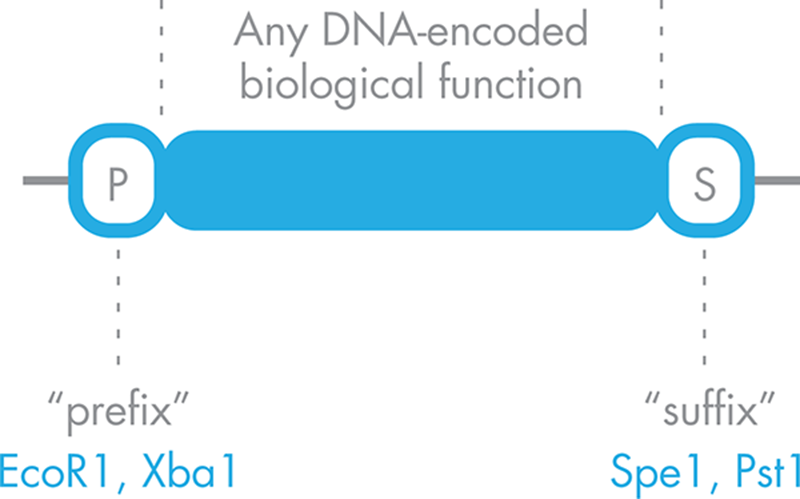
Figure 3-11. A standardized BioBrick part. A DNA-encoded function is shown in blue, flanked by a standardized prefix sequence, “P,” that carries with it two known restriction sites and a standardized suffix sequence, with two different restriction sites.

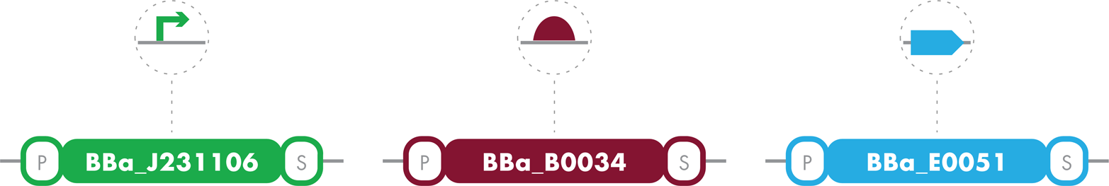
To illustrate this strategy we can consider the building of an iTunes plasmid with the following BioBrick parts:

§ BBa_J231106 = a “medium-strength” promoter

§ BBa_B0034 = a “strong” RBS

§ BBa_E0051 = a modified version of the lacZ gene.

It’s worth mentioning that if our assembly included a DNA segment that does not appear in the Registry, we would need to add several steps to the process to make that DNA into a standardized BioBrick part before moving on to subsequent steps. This requirement illustrates an aspect about standardization we considered earlier in this chapter, namely how standardization generally takes time and energy up front but it can prove more efficient in the long run.

Two assembly steps are needed to put the three parts together. Because order of the parts in the final DNA assembly is important, it’s essential to decide at the outset which parts to cut, and in what order. A number of options could work, but for this example let’s assume that we’ve decided to begin by putting the strong RBS (BBa_B0034) upstream of the lacZ gene (BBa_E0051). As is illustrated in Figure 3-12, the plasmid containing BBa_B0034 could be cut in the part’s prefix with EcoRI and in the part’s suffix with SpeI. In a separate reaction, the plasmid containing BBa_E0051 could be cut in that part’s prefix with XbaI and in its suffix with PstI. Finally, a destination plasmid, where the new assembly will be housed, could be cut with EcoRI so that it’s ready to match up with the prefix of BBa_B0034 and with PstI, making it ready for the suffix of part BBa_E0051.

When you combine and ligate these three DNA fragments, as illustrated in Figure 3-13, the resulting plasmid carries a new composite part BBa_B0034+E0051, which you can give a new part number: BBa_Xnnnnn. This new part conforms to the BioBrick standard in that it has a standard BioBrick prefix, a “mixed” site between the original B0034 and E0051 parts, and is followed by the standard BioBrick suffix. The mixed site between the original parts is no longer recognized by either SpeI or XbaI. Instead, the B0034+E0051 composite part is effectively a new BioBrick. You can enter it into the Registry with a new part number and combine it with any other BioBrick, as shown in Figure 3-14.

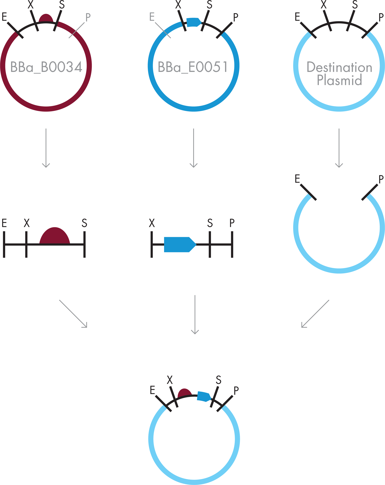
Figure 3-12. BioBrick assembly. BioBrick assembly requires digestion of the plasmid containing the upstream part with EcoRI and SpeI, digestion of the plasmid containing the downstream part with XbaI and PstI, and digestion of the destination plasmid with EcoRI and PstI. These pieces are then combined and ligated to create a plasmid carrying the new BioBrick part.

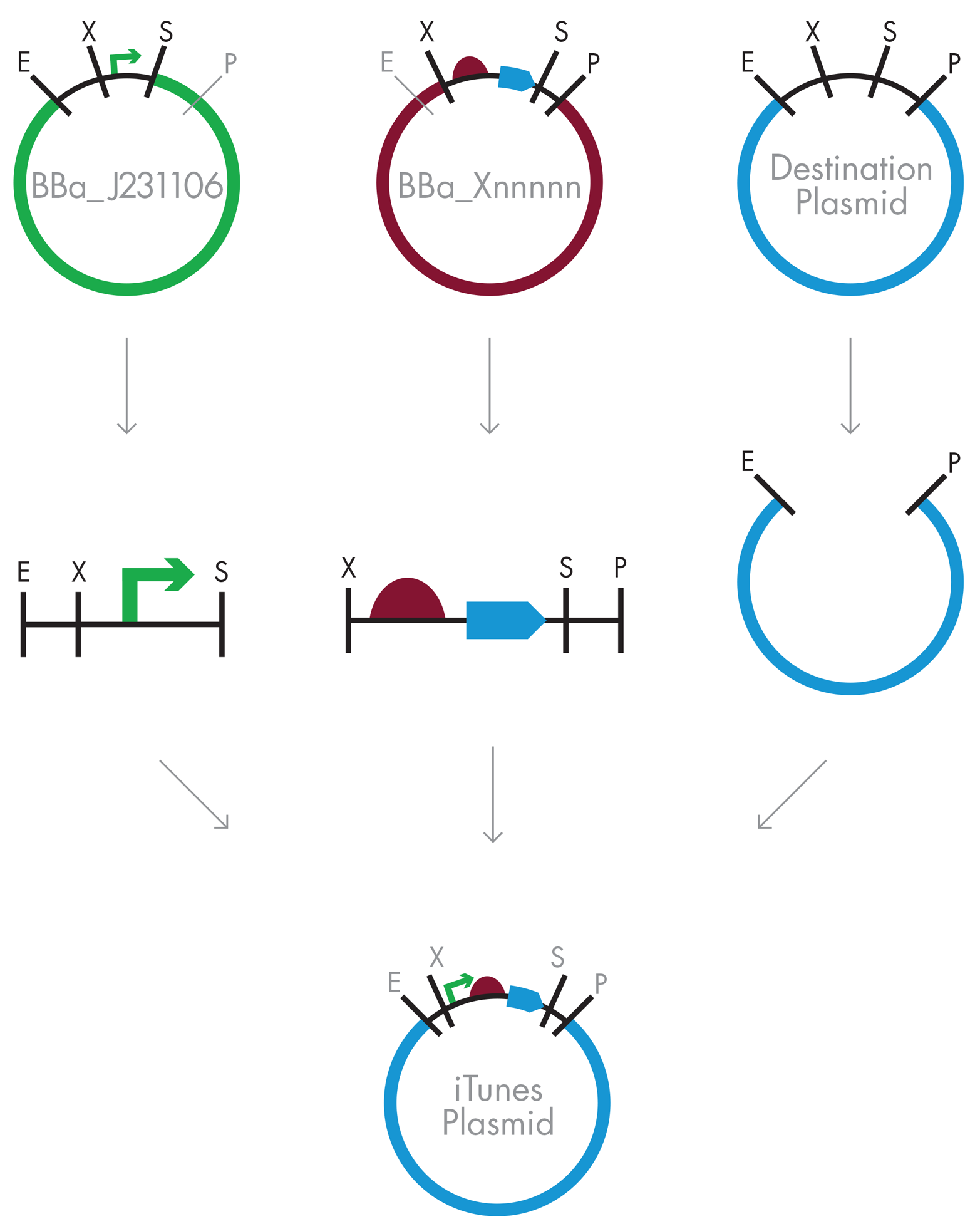
Figure 3-13. BioBrick assembly of composite parts. The strategy to combine standardized BioBrick parts does not change even when the downstream part is a composite part that has been assembled from other basic parts. This is a key enabling feature of BioBrick Assembly methods.

The BioBrick standard streamlines the DNA assembly process when compared with traditional cloning and allows for a reliable, uniform strategy to piece together segments of DNA. Part of the increased efficiency of BioBrick assembly is due to the efforts of others who have standardized the parts beforehand and contributed them to a shared resource. To be useful, the BioBrick parts must be refined so that they carry the expected prefix and suffix and so that they never have any restriction sites from the prefix and suffix within the parts themselves. The refinement process isn’t trivial and does require work. You can introduce the needed changes to the DNA sequence through a technique from the molecular biologists toolkit called site-directed mutagenesis, or through direct chemical synthesis of DNA. Either way, the work that’s required demands an investment of energy and is a barrier to adoption of this standard. Perhaps that’s one of the reasons that other assembly standards have developed, including the Gibson assembly method that’s described next.

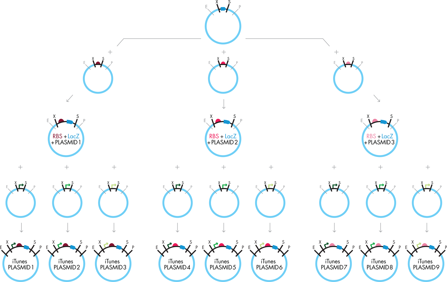
Figure 3-14. Scaling BioBrick assembly. To create the entire iTunes library, you can combine the ORF BioBrick with the three different RBS BioBricks in parallel. You can then separate the resulting composite BioBrick parts into three batches, each of which will be combined with a different promoter to produce the final composite BioBrick parts. As with traditional cloning, you must transform each new composite BioBrick part into E. coli and grow it so that the DNA can be extracted and verified before you can use it as starting material for the next assembly step.

Building DNA: Gibson assembly

Gibson assembly has several advantages over both traditional cloning and BioBrick assembly methods, the greatest of which might be its usefulness for assembling many DNA parts simultaneously. Even in its earliest stage of development, a single Gibson assembly reaction can piece together about ten DNA parts. Thus, this technique represents a huge increase in efficiency over the other DNA assembly methods described, and can be especially useful when assembling complex genetic programs that have more parts and more variations than found in the iTunes plasmid collection we’ve been considering here.

Developed by Dr. Daniel Gibson at the J. Craig Venter Institute during their work on full genome assembly, the Gibson technique uses PCR to prepare multiple DNA fragments for simultaneous assembly (Figure 3-15). The PCR step both generates enough DNA to work with and modifies each DNA part with short sequences that overlap with its partnered part in the final assembly. The overlapping sequences with its intended neighboring part must be at least 25 base pairs for this technique to work. In a second step, the PCR products are pasted together based on the overlapping sequences that have been introduced. No restriction enzymes, or their cognate restriction sites, are required. Instead, a commercially available enzyme, an exonuclease, trims back one of the strands on each DNA part, leaving a DNA overhang on both ends of the fragments. The exonuclease has no sequence specificity; it simply chews back any linear piece of double-stranded DNA moving from the 3′ to 5′ direction. This reaction reveals the customized “sticky ends” that were introduced by the PCR amplification of each DNA part.

Applying this technique to the assembly of an iTunes plasmid (Figure 3-16) presents a challenge because some of the parts in the iTunes DNA assembly are very short. BBa_B0034, the strong RBS, is only 12 base-pairs long, for example. It’s possible to use PCR to append this short RBS sequence with 25 bases of overlap to the promoter on its upstream side and 25 bases of overlap with the lacZ gene on its downstream side. This short RBS part, though, even with the 25 bases on each end, is unlikely to survive the exonuclease treatment. There’s a good chance that it would be chewed back to nothing! Some workaround strategies are possible, but these turn the DNA assembly effort back into an experiment rather than a robust and reliable “go to” technique. In addition, because you must custom build the overlapping sequences between each part for each assembly, putting DNA together with this technique can feel like it’s the experiment, rather than a standardized tool for engineering.

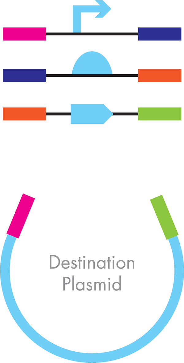
Figure 3-15. Gibson assembly. The different parts of the desired final plasmid include the functional parts—promoter, RBS, and ORF—are shown in light blue. The engineered flanking sequences that guide the order and orientation for assembly are signified by the colored bars.

Figure 3-16. An iTunes plasmid constructed through Gibson-assembly. One of the final DNA constructs is shown with the colored bars between the parts representing the parts of the sequences that were engineered to overlap so that they could be attached to one another in order in a single assembly reaction.

What’s Next?

Biology is inherently variable and changing, but engineers want predictable and functional behavior. To bridge this gap, some creative design thinking is needed. The most attractive designs are likely to harness biology’s unique properties to self-assemble, to reuse a cell’s molecules as building blocks, and to build with precision. The emphasis in this chapter has been on the engineering principle of standardization as it applies to DNA assembly techniques. For every assembly technique described here, there are several more that were not included but that might eventually prevail as the standard for the field. The diversity of approaches speaks to the innovative ideas this challenge is attracting and to the absence of a perfect solution (for now!).

Over time, though, the questions themselves might evolve. Design thinking often ends up asking questions that are different at the end of the process than they were at the beginning. For instance, if you ask for a truckload of three-legged stools so that the workers in your factory can have a place to sit down, you might find it’s the work schedule that actually needed to be changed and you’d have been better off with shorter work shifts and less-tired workers rather than a set of chairs. No one imagined the ohm standard when they started talking about the laying of the trans-Atlantic cables and perhaps no one has yet imagined the best way to engineer DNA or biology.

Additional Reading and Resources

§ Alberts, B. et al. Molecular Biology of the Cell, 4th ed. New York: Garland Science, 2002. Open access: http://bit.ly/mol_bio_of_the_cell.

§ Gibson, D.G. et al. Enzymatic assembly of DNA molecules up to several hundred kilobases. Nature Methods 2009;6:343-5.

§ Knight, T. Idempotent Vector Design for Standard Assembly of Biobricks. DSpace@MIT Citable URI 2003: (http://hdl.handle.net/1721.1/21168).

§ Website: History of the Atlantic Cable & Undersea Communications (http://atlantic-cable.com/).

§ Website: Josephine Cochrane, inventor of the dishwasher (http://bit.ly/dishwasher_cochran).

§ Website: National Institute of Standards and Technology (http://bit.ly/engineered_bio).