An Introduction to Applied Cognitive Psychology - David Groome, Anthony Esgate, Michael W. Eysenck (2016)

Chapter 9. Decision making

Ben R. Newell

9.1 MAKING DECISIONS

This book is concerned with applying what we have learnt to ‘real-world’ situations through the psychological study of cognition. Given this focus, the motivating questions for this chapter on decision making are:

1 What do we know about how people make decisions?

2 How can we apply this knowledge to help people improve their decision making?

Answering the first question requires an understanding of how experimental psychologists study decision making. Answering the second question requires an understanding of how the insights from these studies can be translated into effective strategies for good decision making. But before answering either, we need to think about exactly what we mean by a ‘decision’, and even more importantly what we mean by a ‘good decision’.

A decision can be defined as a commitment to a course of action (Yates et al., 2003); thus researchers with an interest in decision making often ask questions such as: How do people choose a course of action? How do people decide what to do when they have conflicting goals? Do people make rational choices? In psychological research, a distinction is often drawn between a decision (as defined above) and a judgement. A judgement is often a precursor to a decision and can be defined as an assessment or belief about a given situation based on the available information. As such, psychologists with a specific interest in the cognitive processes underlying judgement want to know how people integrate multiple sources of information to arrive at an understanding of, or judgement about, a situation. Judgement researchers also want to know how accurate people’s judgements are, how environmental factors such as learning and feedback affect judgement ability, and how experts and novices differ in the way they make judgements. We will examine examples from both research traditions throughout the course of the chapter, because both offer insights into how to improve performance in real-world environments.

WHAT MAKES A DECISION GOOD?

Take a moment to think about some decisions that you have made in the past year. What comes to mind? The decision to go the beach for your last holiday? The decision about which university to attend? Your decision to take the bus or the train this morning; or perhaps simply the decision to keep reading this chapter? How would you categorise these decisions - ‘good’ or ‘bad’? More generally, how do we assess decision quality?

Yates et al. (2003) examined this question by asking participants to do what you just did - think about a few decisions from the past year. Their participants, who were university undergraduates, then rated the decisions on scales of ‘quality’ (goodness/badness) and ‘importance’, in both cases making the judgements ‘relative to all the important decisions you have ever made’. Table 9.1 displays the quality and importance scores elicited from the participants. Two features stand out: first, good decisions are rated as higher on the quality dimension than bad ones, and are also further from the neutral point (0), suggesting that good decisions are better than bad decisions are bad; second, participants rated their bad decisions as significantly less important than their good decisions.

Table 9.1 Ratings of the quality and importance of real-life decisions

Note: Adapted from data reported in Yates et al. (2003).

When queried further, by far the most often cited reason for why a decision was classified as good or bad was that the ‘experienced outcome’ was either adverse or favourable. Eighty-nine per cent of bad decisions were described as bad because they resulted in bad outcomes; correspondingly, 95.4 per cent of good decisions were described as good because they yielded good outcomes. Other categories identified in questioning were ‘options’, in which 44 per cent of bad decisions were thought to be bad because they limited future options (such as a career-path), and ‘affect’, in which 40.4 per cent of good decisions were justified as good because people felt good about making the decision, or felt good about themselves after making it. These data suggest that our conception of quality is multifaceted, but is overwhelmingly dominated by outcomes: a good decision is good because it produces good outcomes, while bad decisions yield bad ones (Yates et al., 2003).

But how far can such introspection get us in understanding what makes a decision good or bad? Can an outcome really be used as a signal of the quality of the decision that preceded it? Recall one of the decisions suggested earlier - the decision about whether to keep reading this chapter. That cannot be evaluated on the outcome - because you have not read the chapter yet(!) - so you need to make some estimate of the potential benefits of continuing to read. Assessments of the quality of a decision obviously need to take this prospective element of decision making into account. How is this done?

Imagine that you were asked to make an even-money bet on rolling two ones (‘snake eyes’) on a pair of unloaded dice (see Hastie and Dawes, 2001). An even-money bet means that you are prepared to lose the same amount as you could win (e.g. $50 for a win and $50 for a loss). Given that the probability of rolling two ones is actually 1 in 36 (i.e. a one out of six chance of rolling a 1 on one die multiplied by the same chance of rolling a 1 on the other die), taking an even-money bet would be very foolish. But if you did take the bet and did roll the snake eyes, would the decision have been a good one? Clearly not; because of the probabilities involved, the decision to take the bet would be foolish regardless of the outcome.

But would it always be a poor bet? What if you had no money, had defaulted on a loan and were facing the prospect of being beaten up by loan-sharks? Now do you take the bet and roll the dice? If your choice is between certain physical harm and taking the bet, you should probably take it. Thus, not only is the quality of a decision affected by its outcome and the probability of the outcome, it is also affected by the extent to which taking a particular course of action is beneficial (has utility) for a given decision maker at a given point in time (Hastie and Dawes, 2001).

In essence, we can think of these elements - outcomes, probability and utility or benefit - as being at the heart of the analysis of decision making. Theories about exactly how these elements are combined in people’s decisions have evolved in various ways over the past few centuries. Indeed, seventeenth-century ideas based on speculations about what to do in various gambling games (Almy and Krueger, 2013) grew by the middle of the last century into fully fledged theories of rational choice (von Neumann and Morgenstern, 1947).

The details of all of these developments are beyond the scope of this chapter (see Newell et al., 2015 for a more in-depth treatment), but the basic idea can be illustrated by returning to the decision about reading this chapter. Let’s imagine a situation in which you want to decide between continuing to read this chapter and going outside to play football. Let’s also imagine that there are two ‘states of the world’ relevant to your decision - it could rain, or the sun could come out. There are then four possible outcomes: (i) go outside and the sun comes out, (ii) go outside and it rains, (iii) stay in reading and hear the rain battering on the window, (iv) stay in reading and see the sun blazing outside.

A decision-theoretic approach (e.g. von Neumann and Morgenstern, 1947; Savage, 1954) requires that people can assign utilities to the different outcomes involved in a decision. These do not need to be precise numerical estimates of utility; but people should be able to order the outcomes in terms of which they most prefer (with ties being allowed), and express preferences (or indifference) between ‘gambles’ or prospects involving these outcomes. Thus in the reading example you might rank outcome (i) highest (because you like playing football in the sun) and (iv) lowest, but be indifferent between (ii) and (iii).

In addition, this approach requires decision makers to assign probabilities of different outcomes that are bounded by 0 (= definitely will not happen) and 1 (= definitely will happen), with the value of 1/2 reserved for a state that is as equally likely to happen as not. Moreover, the probabilities assigned to mutually exclusive and exhaustive sets of states should sum to 1. Thus if you think there is a 0.8 chance that it will rain, you must also think there is a 0.2 chance that it won’t (because 0.8 + 0.2 = 1).

It is important to note that the elements that make up this representation of a decision problem are subjective, and may differ from individual to individual. Thus your assignment of probabilities and utilities may differ from your friend’s (who might not like football). However, the rules that take us from this specification to the ‘correct’ decision are generally considered to be ‘objective’, and thus should not differ across individuals. The rule is that ofmaximising expected utility (MEU).

Thus the expected utility of each act a decision maker can take (e.g. continue reading) is computed by the weighted sum of the utilities of all possible outcomes of that act. The utility of each outcome is multiplied by the probability of the corresponding state of the world (rain or sun, in this example), and the sum of all these products gives the expected utility. Once the expected utility of each possible act is computed, the principle of MEU recommends, quite simply, that the act with the highest value is chosen.

MAXIMISING MEU IN PRACTICE

But what does this mean in practice? How can we develop these ideas about utility, probability and outcomes into methods for improving decision making? For example, could you use the notion of maximising expected utility to help you decide between two university courses that might be on offer? Let’s assume that next year you can take a course on decision sciences, or a course on physiological psychology. The courses are offered at the same time, so you cannot take both, but either one will satisfy your degree-course requirements. How do you decide?

One way would be to use a technique called multi-attribute utility measurement (often called MAU for short) (Edwards and Fasolo, 2001). The core assumption of MAU is that the value ascribed to the outcome of most decisions has multiple, rather than just a single attribute. The technique employed by MAU allows for the aggregation of the valueladen attributes. This aggregated value can then act as the input for a standard expected utility maximising framework for choosing between alternatives (as outlined briefly in the chapter-reading example).

The first step in using this technique would be to identify the attributes relevant to the decision. These might include whether you think you will learn something, how much work is involved and whether you like the professors teaching the course. Each of these attributes would need to be weighted in order of importance (e.g. are you more concerned about the amount of work or how well you get on with the professor?). The final step requires you to score each of the two courses on a 0-100 scale for each attribute. For example, you might rate decision sciences as 78 but physiological psychology as 39 on the ‘how much do I like the professors’ attribute, reflecting a dislike for the professor teaching the latter course. With these numbers in hand, you could compute the MAU for each course by multiplying the weight of each attribute by its score and summing across all the attributes.

To many of us the MAU procedure might seem rather complicated, time consuming and opaque (How exactly are the weights derived? How do we decide what attributes to consider?). Perhaps pre-empting these kind of criticisms, Edwards (Edwards and Fasolo, 2001) justifies the use of the MAU tool by recounting a story of when a student came to him with a ‘course-choice dilemma’ exactly of the kind just described. Edwards reports that the whole procedure, including explanation time, took less than 3 hours to complete. Moreover, MAU analysis provided a clear-cut result and the student said she intended to choose the recommended course; history does not relate whether she actually did (or whether she thought it was a good decision!).

The MAU tool is widely applicable and could be used in different situations, such as buying a car, choosing an apartment to rent, deciding where to invest your money, even the decision to marry. In all of these situations options can be defined (e.g. cars, financial institutions, people), attributes elicited (e.g. engine type, account type, sense of humour) and weighted for importance, and scores assigned to each attribute - just like in the student’s course example. In this way, the MAU method provides a clear and principled way to make good, rational, decisions. Indeed, there are examples of famous historical figures employing similar techniques in making their own decisions. For example, Darwin is said to have drawn up a primitive form of multi-attribute analysis in attempting to decide whether to marry his cousin Emma Wedgwood. He weighed up the ‘pros’ of attributes such as having a companion in old age against the ‘cons’ of things such as disruption to his scientific work (Gigerenzer et al., 1999). Similarly, the polymath Benjamin Franklin once advocated the use of a ‘moral algebra’, which bears many similarities to modern decision-theoretic approaches, when corresponding with his nephew about job prospects (see Newell et al., 2009).

Such an approach might make sense in many contexts, but there are also clearly many situations in which we simply do not have the time or the necessary knowledge to engage in such careful selection, weighting and integration of information. How do people - particularly ‘in the field’ (or ‘real world’) - make decisions when they do not have the luxury of unlimited time and unlimited information? This is the question asked by researchers who investigate ‘naturalistic decision making’.

9.2 NATURALISTIC DECISION MAKING

Zsambok provides a succinct definition of naturalistic decision making (NDM): ‘NDM is the way people use their experience to make decisions in field settings’ (Zsambok, 1997, p. 4). NDM emphasises both the features of the context in which decisions are made (e.g. ill-structured problems, dynamic environments, competing goals, high stakes, time constraints) (Orasanu and Connolly, 1993), and the role that experience plays in decision making (Pruitt et al., 1997). As such, it is a topic of crucial relevance in examining the application of decision sciences in particular, and cognitive psychology in general, to ‘real-world’ decision making.

According to Klein (1993), a fascinating aspect revealed by cognitive task analyses of professionals making decisions in the field is the lack of decisions they appear to make. There seems to be precious little generation of options or attempting to ‘maximise utility’ by picking the best option; professionals seem to know what to do straightaway - there is no process. Even when one course of action is negated, other options appear to be readily available. Klein claims that the professionals he studies never seem to actively decide anything.

The vignette below, adapted from Klein (1993), which is typical of the kinds of situations that have been analysed in NDM, illustrates these ideas:

A report of flames in the basement of a four-storey building is received at the fire station. The fire-chief arrives at the building: there are no externally visible signs of fire, but a quick internal inspection leads to the discovery of flames spreading up the laundry chute. That’s straightforward: a vertical fire spreading upward, recently started (because the fire has not reached the outside of the building) - tackle it by spraying water down from above. The fire-chief sends one unit to the first floor and one to the second. Both units report that the fire has passed them. Another check of the outside of the building reveals that now the fire has spread and smoke is filling the building. Now that the ‘quick option’ for extinguishing the fire is no longer viable, the chief calls for more units and instigates a search and rescue - attention must now shift to establishing a safe evacuation route.

This description of what the fire-chief does suggests that as soon as he sees the vertical fire he knows what to do - and when that option is not viable he instantly switches to a search and rescue strategy. From a cognitive perspective, what does this ‘instantaneous’ decision making reveal?

The explanation favoured by Klein and colleagues is that experts’ behaviour accords to a recognition-primed decision-making model (RPD; Klein, 1993, 1998). The RPD has three variants (Lipshitz et al., 2001) (see Figure 9.1). In the simplest version a decision maker ‘sizes up’ a situation, recognises which course of action makes sense and then responds with the initial option that is generated or identified. The idea is that a skilled decision maker can typically rely on experience to ensure that the first option generated is a feasible course of action. In a second version of RPD, the decision maker relies on a story-building strategy to mentally simulate the events leading up to the observed characteristics of a situation. Such a strategy is invoked when the situation is not clear and the decision maker needs to take time to carry out a diagnosis. Finally, the third variant (shown in Figure 9.1) explains how decision makers evaluate single courses of action by imagining how they will play out in a given situation. This mental simulation allows the decision maker to anticipate difficulties and amend the chosen strategy.

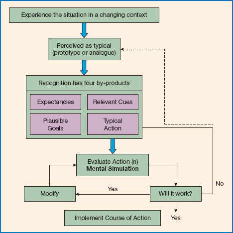
Figure 9.1 The recognition-primed decision-making model.

Source: adapted from Lipshitz et al, 2001.

The RPD model has been applied to a variety of different experts and contexts, including infantry officers, tank platoon leaders and commercial aviation pilots. Consistent with the initial studies of the firefighters, RPD has been shown to be the most common strategy in 80-95 per cent of these environments (Lipshitz et al., 2001). These are impressive results, suggesting that the RPD model provides a very good description of the course of action followed by experienced decision makers, especially when they are under time pressure and have-ill-defined goals (Klein, 1998).

Klein (2009) offers the ‘miracle’ landing of US Airways Flight 1529 on the Hudson River in New York in January 2009 as a compelling example of recognition-primed decision making in action. Klein (2009) suggests that Captain Chesley B. ‘Sully’ Sullenberg III rapidly generated three options when he realised that birds flying into his engines had caused a power failure: (1) return to La Guardia airport; (2) find another airport; (3) land in the Hudson River. Option 1 is the most typical given the circumstances, but was quickly dismissed because it was too far away; option 2 was also dismissed as impractical, leaving the ‘desperate’ but achievable option of ditching in the river as the only remaining course of action. Sully did land in the river, and saved the lives of all on board.

WHAT ABOUT NON-EXPERTS?

The general remit of NDM is decision analysis in ‘messy’ field settings. That is, to describe how proficient decision makers make decisions in the field. Given this focus, the descriptive power of the RPD model is impressive (although one could question its predictive power - i.e. its ability to generate testable hypotheses - cf. Klayman, 2001). But there are also other important considerations for evaluating the insights that the NDM approach offers. For one, its use of experts’ verbal reports as data is perhaps one of the reasons why it appears that no decisions are being made and that everything relies on recognition. Experts - by definition - often have years of experience in particular domains, during which they hone their abilities to generate options, weight attributes and integrate information. Thus, while at first glance they might not appear to be engaging in anything like utility maximising, at some level (of description) they might be. Thus to treat the decisions - or lack thereof - revealed by cognitive task analysis as being completely different from those analysed within a utility maximising framework is perhaps too simplistic.

One could argue that NDM focuses on what some people describe as the more intuitive end of a spectrum bounded by intuition and deliberation (e.g. Hammond, 1996; Hogarth, 2001; Kahneman, 2011). In this context, Herbert Simon’s succinct statement that intuition is ‘nothing more and nothing less than recognition’ (Simon, 1992, p. 155) is a useful insight here (cf. Kahneman and Klein, 2009). Simon’s analogy with recognition reminds us that intuition can be thought of as the product of over-learnt associations between cues in the environment and our responses. Some decisions may appear subjectively fast and effortless because they are made on the basis of recognition: the situation provides a cue, the cue gives us access to information stored in memory, and the information provides an answer (Simon, 1992). When such cues are not so readily apparent, or information in memory is either absent or more difficult to access, our decisions shift to become more deliberative (cf. Hammond, 1996; Hogarth, 2010).

Another way to think about this relation between deliberative and intuitive decisions is that the information relied upon in both cases is the same (or a subset) and that the difference between an expert and novice is the efficiency with which this information can be used, and be used effectively (cf. Logan, 1988). This is why fire-chiefs and pilots undergo extensive training (and why you and I don’t try to fight fires or fly planes!).

Two additional points are worth making. First, there is a tendency in some approaches to studying (or popularising) decision making to equate intuition (in experts) with the involvement of intelligent unconscious processes (e.g. Gladwell, 2005; Lehrer, 2009). Moreover, some researchers suggest we should all rely on unconscious processes (rather than explicit deliberation) when facing complex choices that involve multiple attributes (e.g. Dijksterhuis et al., 2006). This interpretation, and recommendation, is, however, hotly debated. When one undertakes a critical examination of the empirical evidence for ‘genuine’ unconscious influences on decision making (either beneficial or detrimental), the evidence is remarkably weak (Newell, 2015; Newell and Shanks, 2014a). The details of these arguments (and the empirical evidence) are not crucial to our current concerns, but suffice it to say that a healthy dose of scepticism should be applied if you are advised to relax and let your unconscious ‘do the work’ when facing complex decisions.

The second crucial point is that for recognition-primed decision making to be efficient and effective, the right kind of recognition needs to be primed. This might seem like an obvious (even tautologous) claim, but in order to be able to trust our intuitions, or rely on the cues and options that readily come to mind, we need to be sure that we have the appropriate expertise for the environment. Look again at the version of the RPD model shown in Figure 9.1: (appropriate) expertise plays a key role in all three stages of decision making. It is required for recognising the ‘typicality’ of the situation (e.g. ‘it’s a vertical fire’), to construct mental models that allow for one explanation to be deemed more plausible than others, and for being able to mentally simulate a course of action in a situation (deGroot, 1965; Lipshitz et al., 2001). This mental simulation refers to a process by which people build a simulation or story to explain how something might happen, and disregard the simulation as implausible if it requires too many unlikely events.

Klein (1993) points out that when you break the RPD model into these core constituents, it could be described as a combination of heuristics that we rely upon to generate plausible options (e.g. the availability with which things come to mind), to judge the typicality of a situation (e.g. by estimating the representativeness of a given option) - and a simulation heuristic for diagnosis and evaluation of a situation. As we will discover in the next section, the proposals of these and other kinds of judgement heuristics have had an enormous influence on the psychological study of human judgement (Tversky and Kahneman, 1974). Somewhat counterintuitively given the context in which Klein invokes them, the lasting influence has been in terms of the characteristic biases in judgement that they appear to produce.

9.3 HEURISTICS AND BIASES

In 1974, Amos Tversky and Daniel Kahneman published a paper in the journal Science that described three heuristics: availability, representativeness and anchoring. They argued that these heuristics explained the patterns of human judgement observed across a wide variety of contexts. Their evidence for the use of these heuristics came from illustrations of the biases that can arise when people use the heuristics incorrectly. Their approach was akin to the study of illusions in visual perception: by focusing on situations in which the visual system makes errors, we learn about its normal functioning. As we have just seen in the case of naturalistic decision making, many researchers studying applied cognition and decision making readily adopted these heuristics as explanations for phenomena observed outside the psychology laboratory (see the volumes by Kahneman et al., 1982 and Gilovich et al., 2002 for examples, as well as Kahneman, 2011).

The heuristics and biases approach can be explained via appeal to two related concepts: attribute substitution and natural assessment (Kahneman and Frederick, 2002). Attribute substitution refers to the idea that when people are asked to make a judgement about a specific target attribute (e.g. how probable is X?) they instead make a judgement about a heuristic attribute (e.g. how representative is X?), which they find easier to answer. This ease of answering often arises because the heuristic attributes relied upon are readily accessible via the ‘natural assessment’ of properties such as size, distance, similarity, cognitive fluency, causal propensity and affective valence. Kahneman and Frederick (2002) argue that because such properties are ‘routinely evaluated as part of perception and comprehension’ (p. 55), they come more easily to mind than the often inaccessible target attributes. Hence target attributes are substituted for heuristic attributes. Let’s look in a little more detail at each of the three main heuristics identified by Tversky and Kahneman (1974).

AVAILABILITY

Availability, a pervasive heuristic attribute, has been described both as a measure of the ease with which instances come to mind, and as the number of instances that come to mind (Tversky and Kahneman, 1973). Most of the time this heuristic will serve us well as a substitute for estimating frequencies or probabilities - typically more likely events come to mind more readily. However, at times the heuristic will produce errors, and it is these errors that have been the focus of research. Take, for example, a judgement of whether homicide or suicide is more likely in the US adult male population. The majority response is homicide, although in fact suicides are far more common (Lichtenstein et al., 1978). The explanation for this error is simply that instances of homicide come more readily to mind (are more available) than those of suicide. Why? If you don’t know anyone who has committed suicide or homicide, then presumably you either guess or must rely on what you can remember from media coverage/reporting and this is likely to be biased towards homicide because murders are more sensational than suicides.

Note that the biased judgement of homicide arises because of the way in which information is presented to us from external sources (e.g. the media), but availability can also sometimes be a poor guide when we search through simpler information in our memories. Consider this example: What is more probable - that a word starts with the letter k or has k as its third letter? Words with k as the third letter are in fact far more common, but people tend not to give this answer. Tversky and Kahneman (1973) argued that because we tend to organise words by their initial letters - and thus search our memories for them in this way - we tend to think that words starting with k occur more frequently.

REPRESENTATIVENESS

Tversky and Kahneman (1983) gave participants the following simple personality sketch:

Linda is 31 years old, single, outspoken and very bright. She majored in philosophy. As a student, she was deeply concerned with issues of discrimination and social justice, and also participated in anti-nuclear demonstrations.

They then asked separate groups of participants to rank a set of eight statements about Linda either by how representative they appeared to be or how probable they were (e.g. Linda is a bank teller, Linda is a social worker). The correlation between the rankings was 0.99. Tversky and Kahneman took this as very powerful evidence that when people were asked a question about probability, they replaced this target attribute with a heuristic one about representativeness - that is, the degree to which one ‘object’ (Linda in the personality sketch) resembles the ‘object’ of the statement (e.g. Linda is a social worker).

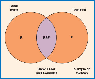
Figure 9.2 Diagram illustrating the Linda problem and the conjunction fallacy.

In another version of the problem (Tversky and Kahneman, 1983), participants were asked: Which of these two statements is more probable? (1) Linda is a bank teller; (2) Linda is a bank teller and active in the feminist movement. The overwhelming majority response was to rank (2) as more probable than (1). This is a clear violation of the conjunction rule of probability: a conjunction cannot be more probable than either of its conjuncts. All feminist bank tellers are, by definition, bank tellers, so a person cannot be more likely to be a feminist bank teller than just a bank teller. The illustration provided in Figure 9.2 is usually sufficient to convince a classroom of students of this fact! Nonetheless, the description of Linda is highly representative of active feminists but not of bank tellers, thus a judgement by representativeness leads to statement (2) receiving the higher ranking.

ANCHORING

Anchoring is the tendency for estimates of continuous variables (e.g. age, height, weight, price etc.) to be affected by the presentation of initial values. The typical anchoring task involves providing a high (or low) anchor to separate groups of participants - e.g. Do you think Gandhi died before or after the age of 140 (or 9) years old? - and then asking for an estimate - e.g. How old was Gandhi when he died?

Anchoring is obtained if the estimate is drawn towards the anchor. Thus participants given a high anchor will estimate a higher value (67 years old, in this case) than those given a low anchor (50 years old) (Strack and Mussweiler 1997). Although anchoring effects might seem at first glance entirely sensible (and indeed it has been argued that anchoring may be a rational response to the implied communicative intent of the experimenter - see Mussweiler and Strack, 1999), they are pervasive even in situations where the individual knows that the anchor value is uninformative. For example, you know, presumably, that Gandhi was neither 9 nor 140 when he died and yet your answer would probably be influenced by the mere presentation of either of those ‘anchor’ numbers.

A considerable body of research has explored two general classes of explanation. In the anchoring-and-adjustment account, first proposed by Tversky and Kahneman (1974), individuals are assumed to take the anchor as a reasonable starting point for their judgement and then move away from it as they retrieve relevant information from memory. However, these adjustments are assumed to be conservative and insufficient (as such, this explanation does not fit readily within the attribute substitution framework, cf. Kahneman and Frederick, 2002). In the selective accessibility model (Strack and Mussweiler, 1997), in contrast, the anchor is assumed to render anchor-consistent features of the target of judgement accessible via a process of semantic activation. Chapman and Johnson (2002) provide a good discussion of the relative merits of these two accounts.

The exact explanation of anchoring need not concern us here, but it is important to note that, just as availability and representativeness appear to be involved in naturalistic decisions (see Figure 9.1), anchoring is also observed outside the laboratory. In an applied setting, Northcraft and Neale (1987) found that anchors (suggested listing prices) influenced the pricing decisions that both non-experts (students) and professional real-estate agents made when they spent 20 minutes viewing a residential property. Real-estate agents who were told in advance that the listing price of the property was $65,900 assessed its value at $67, 811. In contrast, agents told that the same property was listed at $83,900 gave an average appraisal of $75,190. The non-experts showed an even stronger pattern - their appraisal values with the high anchor were almost $10,000 higher than the low anchor.

MIND AND ENVIRONMENT?

The preceding sections all highlight situations in which reliance on shortcuts or heuristic methods for judgement leads to errors. At first glance, these demonstrations sit uneasily with research from naturalistic decision making (Section 9.2) emphasising how useful and adaptive these retrieval, substitution, assessment and simulation techniques can be for people making decisions in the ‘messy’ real world. How can these views be reconciled?

One answer comes from considering not just the cognitive capabilities of the decision maker but also the interaction of these abilities with the environment in which the decision is made (Simon, 1956; Gigerenzer and Gaissmaier, 2011). One characteristic of the questions posed in demonstrations of the availability and representativeness heuristic is that they are carefully crafted to elicit the predicted biases. These experimental tasks and their accompanying instructions often bear little relation to the kinds of situation we often face. For example, responses in famous demonstrations such as the Linda problem (Figure 9.2) can be reinterpreted as sensible rather than erroneous if one uses conversational or pragmatic norms rather than those derived from probability theory (Hertwig et al., 2008; Hilton, 1995). In a similar vein, when more representative samples are used, such as using a large sample of letters rather than only the five consonants that do appear more often in the third than first position of words, ‘availability biases’ such as the ‘letter k’ effect can be shown to disappear (Sedlmeier et al., 1998).

The central message is that judgements and decisions do not occur in a vacuum, and we need to take seriously the interface between the mind of the decision maker and the structure of the environment in which decisions are made (Fiedler and Juslin, 2006). Only then do we appreciate the ‘boundedly rational’ nature of human judgement and decision making. An oft-cited metaphor that emphasises this interaction is Herbert Simon’s scissors: ‘Human rational behavior … is shaped by the scissors whose two blades are the structure of the task environment and the computational capabilities of the actor’ (Simon, 1990, p. 7).

Juslin et al. (2009) offer the following example to give this idea some context: appreciating why a deaf person concentrates on your lips while you are talking (a behaviour) requires knowing that the person is deaf (a cognitive limitation), that your lip movements provide information about what you are saying (the structure of the environment), and that the person is trying to understand your utterance (a goal). The crucial point is that, on their own, none of these factors explains the behaviour or its rationality. These can only be fully appreciated by attending to the structure of the environment - this is the essence of what Simon termed bounded rationality.

ADAPTIVE USE OF HEURISTICS?

As a partial reaction to the overly negative impression of human cognition offered by the heuristics and biases tradition, Gigerenzer and colleagues have championed adaptive ‘fast-and-frugal’ heuristics. At the heart of the fast-and-frugal approach lies the notion of ecological rationality, which emphasises ‘the structure of environments, the structure of heuristics, and the match between them’ (Gigerenzer et al., 1999, p. 18). Thus the concern is not so much with whether a heuristic is inherently accurate or biased, but rather why and when a heuristic will fail or succeed (Gigerenzer and Brighton, 2009). This focus on the ‘ecology’ brings context to the fore and overcomes the perceived ‘cognition in a vacuum’ criticism of the heuristics and biases approach (McKenzie, 2005).

This programme of research has offered an impressive array of heuristics describing how to catch balls (the gaze heuristic), how to invest in the stock market (the recognition heuristic), how to make multi-attribute judgements (the take-the-best heuristic), how to make inferences about our social environment (the social-circle heuristic) and even how to make sentencing decisions in court (the matching heuristic). (See Gigerenzer et al., 2011 for descriptions of these and many other heuristics.) These simple rules for how information in the environment can be searched, when the search should terminate and how one should decide, echo ‘decision-tree’ models that can be employed by professionals who need to make accurate decisions quickly. A good example is the Ottawa ankle rules for deciding whether an ankle is sprained or fractured. A physician adopting these rules asks the patient to walk four steps and asks no more than four questions about the pain and bone tenderness. The rules are extremely successful for determining whether x-rays are required, thereby avoiding unnecessary exposure to radiation for those who have only sprained their ankle (Bachmann et al., 2003; Gigerenzer, 2014; see also Martignon et al., 2003 for a discussion of how fast-and-frugal heuristics relate to fast-and-frugal decision trees, and Jenny et al., 2013 for an application of decision trees to diagnosing depression).

The fast-and-frugal approach to understanding how we make judgements and decisions has not been immune to critique - not least by those questioning whether people actually use such heuristics in practice despite the heuristics’ apparent success in theory (e.g. Dougherty et al., 2008; Newell, 2005, 2011). In other words, although simple rules and decision trees derived from extensive analyses of the relevant databases might lead to accurate predictions in certain settings, the success of these rules reveals little - critics argue - of the way in which people can and do decide when faced with similar tasks. These are of course different questions: the first focuses on the environment and ‘what works’, and the second asks how the mind might implement these successful rules - a cognitive-process-level explanation.

As a brief aside, deciding which of these questions one wants to answer in the context of applied cognition or applied decision making is not always obvious. If our goal is simply to facilitate decision making then, as Larrick (2004) points out, perhaps the ultimate standard of rationality might be being aware of our limitations and knowing when to use superior decision tools, or decision trees (see Edwards and Fasolo, 2001; Newell et al., 2015; Yates et al., 2003 for additional discussion of such decision support techniques).

9.4 LEARNING TO MAKE GOOD DECISIONS

Despite the often antagonistic presentations of research from the heuristics and biases and the fast-and-frugal heuristics traditions (e.g. Gigerenzer, 2014), fundamental conclusions about the importance of well-structured environments for enabling accurate judgements are emphasised by both traditions. For example, Kahneman and Klein (2009) write: ‘evaluating the likely quality of an intuitive judgement requires an assessment of the predictability of the environment in which the judgement is made and of the individual’s opportunity to learn the regularities of that environment’ (p. 515). In other words, when an individual has no opportunity to learn or the environment is so unpredictable that no regularities can be extracted (or both), judgements are likely to be very poor. However, when an environment has some predictable structure and there is an opportunity to learn, judgements will be better and will improve with further experience.

Such conclusions about differences in the quality of expert judgement are supported by studies that have compared expertise across professions. Shanteau (1992) categorised livestock judges, chess masters, test pilots and soil judges (among others) as exhibiting expertise in their professional judgements. In contrast, clinical psychologists, stockbrokers, intelligence analysts and personnel selectors (among others) were found to be poor judges (cf. Meehl, 1986). The reason for the difference again comes back to predictability, feedback, and experience in the different professional environments. Livestock, it turns out, are more predictable than the stock market.

Dawes et al. (1989) give a concrete example of why some environments are more difficult than others for assessing important patterns. Consider a clinical psychologist attempting to ascertain the relation between juvenile delinquency and abnormal electroencephalographic (EEG) recordings. If, in a given sample of delinquents, she discovers that approximately half show an abnormal EEG pattern, she might conclude that such a pattern is a good indicator of delinquency. However, to draw this conclusion the psychologist would need to know the prevalence of this EEG pattern in both delinquent and non-delinquent juveniles. She finds herself in a difficult situation because she is more likely to evaluate delinquent juveniles (as these will be the ones that are referred), and this exposure to an unrepresentative sample makes it more difficult to conduct the comparisons necessary for drawing a valid conclusion.

What about the real-estate experts who appeared to be susceptible to simple anchoring biases in the Northcraft and Neale (1987) study discussed earlier? Why didn’t their experience of buying and selling houses outweigh any potential influence of (erroneous) price listing? Perhaps the real-estate market is not sufficiently predictable for adequate learning from feedback to occur. One interesting feature of the Northcraft and Neale study was that on a debriefing questionnaire, about half of the non-experts but only around a quarter of the real-estate agents reported giving consideration to the anchor in deriving their pricing decisions.

As Newell and Shanks (2014b) discuss, this pattern raises a number of possible interpretations. First, it could be that the anchoring effect in experts was entirely borne by those participants who reported incorporating the anchor into their estimates. Recall that the anchoring effect was smaller in the experts than in the non-experts, and thus consistent with the relative proportion in each sample reporting use of the anchor. Second, the majority of experts might not have been aware of the influence of the anchor on their judgements. This is possible, but as discussed in detail by Newell and Shanks (2014a), it is notoriously difficult to assess awareness exhaustively in these situations. Third, and related to the awareness issue, it may be that the experts were aware of the influence of the anchor but avoided reporting its use because of the situational demands. As Northcraft and Neale (1987, p. 95) themselves put it,

[I]t remains an open question whether experts’ denial of the use of listing price as a consideration in valuing property reflects a lack of awareness of their use of listing price as a consideration, or simply an unwillingness to acknowledge publicly their dependence on an admittedly inappropriate piece of information.

More research investigating how aware experts are of their reliance on biased samples of information or erroneous cues would be very valuable, not least because this work would contribute to understanding optimal ways to debiasjudgement. In the context of anchoring, one debiasing strategy is to ‘consider the opposite’ (Larrick, 2004; Mussweiler et al., 2000). As Larrick (2004) notes, this strategy simply amounts to asking oneself, ‘What are some of the reasons that my initial judgement might be wrong?’ It is effective because it counters the general tendency to rely on narrow and shallow hypothesis generation and evidence accumulation (e.g. Klayman, 1995). As such, it perhaps forces people to consider why using the provided anchor number might be inappropriate. (See also Lovallo and Kahneman, 2003 for the related idea of ‘adopting the outside view’ when making judgements and forecasts).

KIND AND WICKED ENVIRONMENTS?

In a recent set of papers, Hogarth and colleagues have taken a novel approach to understanding why good, unbiased, judgements and decisions arise in some environments but not in others (e.g. Hogarth, 2001; Hogarth and Soyer, 2011, in press; Hogarth et al., in press). Hogarth distinguishes between kind and wicked learning environments and also between transparent and non-transparent descriptions of decision problems. The kindness/wickedness of an environment is determined by the accuracy and completeness of the feedback one receives. If the feedback is complete and accurate, it can help people reach unbiased estimates of the nature of the environment in which they are operating. If it is incomplete, missing or systematically biased, an accurate representation cannot be acquired.

Transparency refers to the ease with which the structure of a problem can be gleaned from a description. Hogarth and Soyer (2011) argue that a problem in which the probability of a single event affects an outcome is relatively transparent, whereas when a probability needs to be inferred from the conjunction of several events, the problem becomes more opaque. By crossing these two dimensions one can develop a taxonomy of tasks or situations that range from the least amenable for accurate judgement, a non-transparent task in a wicked learning environment, to the most amenable, transparency in description and a kind environment.

They demonstrate that combing an opaque description with the opportunity to interact in a kind environment can lead to significant improvements in judgement relative to just providing a description. A good example of these kinds of improvement is provided by considering what has become a notorious illustration of faulty reasoning: so-called ‘base-rate neglect’ problems.

Box 9.1 displays one of the problems often used in these demonstrations (e.g. Gigerenzer and Hoffrage, 1995; Krynski and Tenenbaum, 2007). The task facing the participant is to use the statistical information provided in the description to work out the probability that a woman who receives a positive result on a routine mammogram screening (i.e. a tumour appears to be present) actually has breast cancer.

The way to solve this problem correctly is to use a mathematical formulation known as Bayes’ Rule. This a rule for updating your beliefs on the basis of incoming evidence. Essentially, it works by taking your ‘prior belief’ in a given hypothesis and then modifying this belief on the basis of new information to produce a ‘posterior probability’ or belief in the hypothesis after you have incorporated new information.

In the problem described in Box 9.1, three key statistics are presented: the prior probability, or base rate, of women in the population with breast cancer, p(c) = .01, the likelihood or ‘hit rate’ of the mammogram (M) to detect breast cancer in women with cancer, p(M | C) = .80, and the ‘false-positive rate,’ p(M | -C) = .15 - that is, the likelihood of a tumour being indicated even when no cancer is present (this is what M | -C means). These statistics allow calculation of the target quantity - the conditional probability of breast cancer given a positive mammo gram. Before looking at Box 9.2, which shows how these numbers are entered into Bayes’ Rule to produce the answer, what is your best estimate of this conditional probability? Don’t feel bad if you are guessing or have no idea - you are in good company!

Box 9.1 Description of a reasoning problem used to illustrate ‘base-rate neglect’

Doctors often encourage women at age 50 to participate in a routine mammography screening for breast cancer.

From past statistics, the following is known:

✵ 1% of women had breast cancer at the time of the screening.

✵ Of those with breast cancer, 80% received a positive result on the mammogram.

✵ Of those without breast cancer, 15% received a positive result on the mammogram.

✵ All others received a negative result.

Your task is to estimate the probability that a woman, who has received a positive result on the mammogram, has breast cancer.

Suppose a woman gets a positive result during a routine mammogram screening. Without knowing any other symptoms, what are the chances she has breast cancer?

___%

Box 9.2 The solution to the problem shown in Box 9.1 (using Bayes’ Rule)

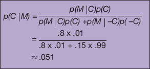
Now take a look at Box 9.2. The correct answer - around .051 or 5 per cent - is probably much lower than your estimate. Most people given these tasks provide conditional probability estimates that are much higher than the correct solution. And it is not just students and non-experts. In one of the early investigations of these problems, students and staff at Harvard Medical School were given an example similar to that shown in Box 9.1 and only 18 per cent got the answer right, with most providing large overestimates (Casscells et al., 1978). So why do people find these problems so difficult?

The standard explanation is that people pay insufficient attention to the base rate - that is, the population prevalence of breast cancer, hence the term base-rate neglect (cf. Evans et al., 2000; Gigerenzer and Hoffrage, 1995). This error can be interpreted in terms of the attribute substitution account discussed earlier (Kahneman and Frederick, 2002). People are faced with a difficult probability problem - they are asked for the probability of cancer given a positive mammogram, and this requires a relatively complex Bayesian computation. However, there is a closely related (but incorrect) answer that is readily accessible, and so they give this. Perhaps the most readily accessible piece of information is the ‘hit rate’ or sensitivity of the test (80 per cent), and so people often simply report that figure. In this case they are substituting the accessible value of the probability of a positive mammogram given cancer, P(M|C), for the required posterior probability, P(C|M).

Several different approaches have been taken in an effort to move people away from making these errors. For example, the natural frequency hypothesis suggests that presenting statistical information as frequencies (e.g. 8 out of 10 cases) rather than probabilities (e.g. .8 of cases) increases the rate of normative performance markedly (e.g. Cosmides and Tooby, 1996; Gigerenzer and Hoffrage, 1995). This approach builds on the ecological rationality idea alluded to earlier, that the mind has evolved to ‘fit’ with particular environments and is better suited to reason about raw, natural frequencies than more abstract probabilities. Building on this basic idea, Gigerenzer (2014) advocates a radical rethinking of the way we teach statistical literacy in schools, claiming that such programmes will turn us into ‘risk-savvy’ citizens.

Alternative approaches emphasise that instructions clarifying set relations between the relevant samples (Barbey and Sloman, 2007; Evans et al., 2000) and provision of causal frameworks for relevant statistics (e.g. Hayes et al., 2014; Krynski and Tenenbaum, 2007) can also lead to substantial improvements in reasoning.

Our current focus, though, is on the improvement that can be obtained by structuring the learning environment appropriately. This approach shares some similarities with the natural frequency hypothesis, but rather than simply redescribing the information in different ways, Hogarth and colleagues emphasise the role of experiential sampling - literally ‘seeing for oneself’ how the problem is structured.

Hogarth and Soyer show that if descriptive information of the kind displayed in Box 9.1 is augmented with an opportunity to sample outcomes from the posterior probability distribution, judgements improve dramatically. Recall that the posterior probability is what the question is asking for: what is the probability that a woman has breast cancer given that she received a positive test? In their experiments this sampling took the form of a simulator offering trial-by-trial experience of ‘meeting different people’ from the population who had a positive test result and either did or did not actually have cancer. Experiencing these sequentially simulated outcomes presumably highlighted the relative rarity of the disease - even in individuals who tested positive - thereby helping people overcome the lack of transparency inherent in the purely described version of the problem. Indeed, virtually all the participants given this opportunity to sample subsequently gave the correct answer.

The exact reason why sampling in this context confers an advantage is still a matter for debate. For example, Hawkins et al. (2015) showed that sampling from the prior distribution (i.e. the base rate) did not lead to improved estimates, despite the fact that this form of sampling should reinforce the rarity of cancer in the population. Moreover, Hawkins et al. found that providing a simple (described) tally of the information that another participant had observed via active sampling led to the same level of improvement as trial-by-trial experience.

These issues, and others concerning how one should best characterise ‘kind’ and ‘wicked’ learning environments, remain important questions for future research (e.g. Hogarth et al., in press). Nevertheless, the central message that these kinds of simulation methodologies can improve understanding is gaining traction in a wide variety of applied contexts, from financial decisions (Goldstein et al., 2008; Kaufmann et al., 2013) to understanding the implications of climate change (Newell et al., 2014; Newell and Pitman, 2010; Sterman, 2011) to helping business managers make forecasts (Hogarth and Soyer, in press).

9.5 RATIONALITY UNDER RISK?

Earlier in the chapter we discussed how the study of decision making involves thinking about outcomes, probabilities and utility or value. A rational choice is deemed to be one that maximises a person’s utility given a set of outcomes and their associated probabilities. We used the decision about whether to continue reading this chapter as an illustrative example (hopefully a decision you now consider ‘good’), but often researchers use simple monetary gambles with clearly specified outcomes and probabilities in order to test theories about how people choose and whether those choices are rational.

One very influential theory of this kind is prospect theory (Kahneman and Tversky, 1979). Figure 9.3(a) shows a typical gamble problem used to test prospect theory. Participants are asked to imagine choosing between a certain gain of $3000 or a gamble involving an 80 per cent chance of gaining $4000 or a 20 per cent chance of receiving nothing. What would you choose? If you chose according to a simple expected value calculation, you would take the gamble, because $4000 multiplied by 0.8 is $3200 which is higher than $3000. But as the graph in Figure 9.3(a) clearly illustrates, the overwhelming preference in this gamble is for the ‘sure thing’ - the $3000. Kahneman and Tversky (1979) interpreted this pattern of choice as indicating a ‘certainty effect’ - that people tend to overweight certain outcomes relative to merely probable ones. Another way to think about the choice pattern is that people might overweight the 20 per cent chance of getting nothing in the gamble and therefore avoid it.

What happens if one faces losses rather than gains? Kahneman and Tversky (1979) found that if the problem shown in Figure 9.3 was changed to a certain loss of $3000 or a gamble with an 80 per cent chance of losing $4000 and a 20 per cent chance of losing nothing, preferences reversed completely. Now 92 per cent of their participants took the gamble! This switch in preferences can be interpreted in the same way: people overweight certainty - and don’t like losses - so they avoid the sure thing, and they also overweight the possibility that they might lose nothing (the best outcome) if they take the gamble.

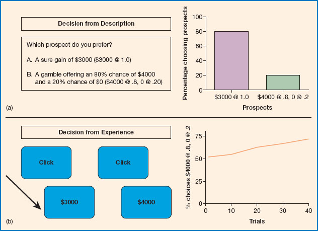
Figure 9.3 Risky choices from description (a) and experience (b). Note: In (a), where probabilities and outcomes are provided in a description, the majority prefer the sure thing ($3000). In (b), where probabilities and outcomes are learnt via experience, people develop a preference for the risky alternative ($4000 with an 80 per cent chance and $0 with a 20 per cent chance) over the trials of the experiment. In the example, a participant has clicked once on the left button and seen an outcome of $3000, and once on the right button and seen $4000. On some occasions (about 20 per cent of clicks) the right button reveals the $0 outcome, but despite this, people tend to choose as if they underweight the rarer 0 outcome and choose this riskier option more often.

The figures are illustrative and adapted from data reported in Kahneman and Tversky (1979; a) and Barron and Erev (2003; b).

Patterns of choices like these and several others led Kahneman and Tversky to develop a psychological theory of choice under risk that was still deeply rooted in the underlying logic of maximising expectation - but proposed crucial modifications whereby both the utilities and probabilities of outcomes undergo systematic cognitive distortions. The details of these cognitive distortions need not concern us here (for more in-depth reviews see Newell, 2015 and Newell et al., 2015), but we should note that the concepts derived from prospect theory have been very influential in attempts to understand decision making outside the psychology laboratory (see Camerer, 2000 for several examples).

One good example is a study by Pope and Schweitzer (2011), who argue that a key tenet of prospect theory - loss aversion - is observed in the putting performance of professional golfers. In an analysis of 2.5 million putts, Pope and Schweitzer demonstrate that when golfers make ‘birdie’ putts (ones that would place them 1 shot below par for the hole - a desirable result), they are significantly less accurate than when shooting comparable putts for par. Specifically, they tend to be more cautious and leave the ball short of the hole. Such behaviour is interpreted as loss aversion, because missing par (taking more shots to complete a hole than one ‘should’) is recorded as a loss relative to the normative ‘par’ reference point and thus golfers focus more when they are faced with a putt to maintain par. (Note that this pattern would also be consistent with the slightly different notion of loss attention rather than aversion - see Yechiam and Hochman, 2013.)

NUDGING PEOPLE TO BETTER CHOICES?

Although debate remains about the prominence and relevance of biases seen in the lab for behaviour observed in the real world (e.g. Levitt and List, 2008), the work on prospect theory is credited as the watershed for the discipline now known as behavioural economics. Behavioural economics - the study of human economic behaviour - as opposed to that of a strictly rational economic agent - is currently enjoying a heyday. Several governments (US, UK, Australia) are seeking policy advice from psychologists and economists who have developed behavioural ‘nudges’ based on simple insights from prospect theory, such as the differences in reactions to gains and losses, and the desire for the status quo (e.g. John et al., 2011; Thaler and Sunstein, 2008).

The basic premise of the ‘nudge’ approach is that our decisions are influenced by the ‘choice architecture’ in which we find ourselves. The way that options are presented on a screen, or the way that food is arranged in a canteen, can all ‘nudge’ us towards making particular choices. Take the example of organ donation (Johnson and Goldstein, 2003). In some countries, such as Austria, the default is to be enrolled as an organ donor - there is a presumed consent that you are willing to donate your organs in the event of your death. In other countries, such as Germany, you have to make an active decision to become a donor. Johnson and Goldstein found that this setting of the default had a profound effect on the rates of organ donation. For example, although Austria and Germany are similar countries in terms of socio-economic status and geographic location, only 12 per cent of Germans were donors (in 2003) compared with 99.98 per cent of Austrians.

Johnson and Goldstein explain this huge difference in terms of the choice architecture: when being a donor is the ‘no-action’ (status quo) default, almost everyone consents (i.e. in Austria), but when one needs to take action, because the choice architecture is not conducive, consent rates are much lower (i.e. in Germany). The effect of defaults might not only be driven by the extra effort of opting in - factors such as implied endorsement and social norms (‘if that option is already selected perhaps that is what I should do’) and the sense of loss from giving up a chosen option might also contribute (Camilleri and Larrick, 2015).

Defaults are but one aspect of choice architecture. Camilleri and Larrick (2015) discuss information restructuring and information feedback as other tools at the choice architect’s disposal. The former refers simply to the way in which choice attributes and alternatives can be presented in order to highlight particular aspects of the choice environment, the latter to the idea that tools can present real-time feedback to users to guide choices and behaviour. Camilleri and Larrick identify several situations from the environmental domain - such as describing the fuel efficiency of vehicles and tools for monitoring energy use - that take advantage of psychological insights.

Whether the current level of interest in nudges and behavioural economics more generally will be sustained remains to be seen. Some argue that the idea of a ‘benevolent’ choice architect designing environments to encourage particular choices has Orwellian overtones that encroach on our freedom (The Economist, 2014). One interesting recent development in this area is the proposal by proponents of the simple heuristics approach discussed earlier (e.g. Gigerenzer et al., 1999) of their own brand of decision improvement ‘tools’. The contrast between what these authors term ‘boosting’ and nudging is summarised by Grüne-Yanoff and Hertwig (in press, p. 4) as follows:

The nudge approach assumes ‘somewhat mindless, passive decision makers’ (Thaler and Sunstein 2008, p. 37), who are hostage to a rapid and instinctive ‘automatic system’ (p. 19), and nudging interventions seek to co-opt this knee-jerk system or behaviors such as … loss aversion … to change behavior. The boost approach, in contrast, assumes a decision maker whose competences can be improved by enriching his or her repertoire of skills and decision tools and/or by restructuring the environment such that existing skills and tools can be more effectively applied.

Once again the importance of thinking about the interface between the mind and the environment is emphasised in this approach. Whether it be the ‘science of nudging’ or the ‘science of boosting’ (or both) that take off, there is no doubt that these applications represent real opportunities for findings from the psychology lab to have impacts in the domains of health, environment and social welfare.

LEARNING AND RISKY CHOICES

Whether one tries to redesign a choice architecture in order to ‘nudge’ people to make choices, or to ‘boost’ the competencies they already have, an important factor to consider is that preferences and choices can change over time as people learn about the environment in which they are making decisions. The research on probability judgement discussed earlier (e.g. Hogarth and Soyer, 2011) reminds us that sampling or simulation of the potential outcomes changes judgement; similarly, recent research on what has become known as ‘decisions from experience’ has suggested a reconsideration of how people make risky choices.

The standard ‘decision from experience’ experiment is very simple and is summarised in Figure 9.3(b). Participants are presented with two unlabelled buttons on a computer screen and are asked to click on either one on each trial of a multi-trial experiment. A click on the button reveals an outcome that the participant then receives; the probability of the outcome occurring is pre-programmed by the experimenter but the participant does not know what the probability is - she has to learn from experience. In the example in Figure 9.3, the participant learns over time that one button pays out $3000 every time it is clicked and the other $4000 on 80 per cent of clicks and 0 on 20 per cent (these are hypothetical choices, or often in terms of pennies rather than dollars!). Recall that when this problem is presented in a described format, the overwhelming preference is for the certain reward ($3000) (see Figure 9.3(a)). What happens when the same problem is learnt via experience from feedback? Contrary to the dictates of the certainty effect, participants now come to prefer the $4000 button (Barron and Erev, 2003). The graph in Figure 9.3 shows this pattern - across the forty trials of an experiment, participants start to click more and more on the button representing the gamble (the orange line increases across trials, indicating a greater proportion of choices for that button).

Furthermore, if the prospects are converted into losses, so now one button offers -$3000 on every click and the other -$4000 on 80 per cent of clicks, participants learn to prefer the certain loss of $3000. In other words, under experience there is a striking reversal of the certainty effect and participants appear to be risk seeking in the domain of gains and risk averse in the domain of losses - the opposite of what influential theories of decisions from simple descriptions predict (e.g. prospect theory). One way to explain this pattern is by assuming that in decisions from experience, people tend to underweight the smaller (i.e. 20 per cent) probability of getting nothing in the gain frame - leading to a choice of the $4000, .80 - and similarly underweight the smaller possibility (20 per cent) of losing nothing in the loss frame - leading to a choice of the $3000. In essence, where prospect theory predicts overweighting, we see underweighting.

These and many other differences in the patterns of choice between described and experienced decisions have led some authors to suggest a rethink of how many everyday risky choices are made (e.g. Erev and Roth, 2014; Rakow and Newell, 2010). The simple insight that people tend to underweight rare events in decisions from experience has important implications. One example is in attempts to ensure that people use safety equipment, or conduct safety checks. In such cases Erev and Roth (2014) suggest that explanation (description) of the relevant risks might not be enough to ensure safe practices. They give the example that informing people that yearly inspections of motor vehicles are beneficial because they reduce the risk of mechanical problems and accidents may not be enough. This is because when people make decisions from experience, they are likely to underweight these low-probability but high-hazard events and behave as if they believe ‘it won’t happen to me’ (see also Yechiam et al., 2015) (just as they behave as if they believe they won’t receive the 0 outcome in the problem shown in the lower half of Figure 9.3). Thus yearly inspections need to be mandated rather than just encouraged.

9.6 CONCLUSIONS

The psychological study of judgement and decision making is incredibly rich and diverse. Here we have barely scratched the surface but hopefully you will have gained some insights into how the results of theoretical analyses and simple laboratory experiments can inform daily decision making in the ‘messy’ real world. Two key take-home messages from this brief overview are (1) to take the interface between the capabilities of the mind and the structure of information in the environment seriously. This is particularly important in situations where we need to assess the quality of expert judgements and to assess whether we have the right kind of expertise for a given decision. (2) Judgements and decisions do not arise from thin air - we learn from experience, and the nature of that learning, and the nature of the environment in which that learning occurs, have crucial implications for the quality of our decisions (cf. Newell et al., 2015).

SUMMARY

✵ A decision can be defined as a commitment to a course of action; a judgement as an assessment or belief about a given situation based on the available information.

✵ Formal approaches to assessing decision quality incorporate ideas about outcomes, probabilities and benefit (or utility), and prescribe a utility maximisation calculus.

✵ Naturalistic decision making (NDM) examines how people use experience to make judgements and decisions in the field. The approach emphasises the importance of recognition-primed decision making.

✵ NDM, in turn, is built on notions of judgement heuristics - availability, representativeness, anchoring - and the characteristic biases that can occur due to (at times) inappropriate reliance on such rules of thumb.

✵ A different class of heuristics - fast and frugal - emphasise the need to consider the boundedly rational nature of human cognition and the importance of the interaction between the mind and the environment.

✵ This crucial mind · environment interaction highlights the role of learning from feedback in well-structured (kind) environments and the differences that can occur when people make decisions on the basis of described or experienced (sampled) information.

✵ The psychological study of judgement and decision making is replete with important applications to real-world problems and situations, and further research elucidating how, why and when expertise ‘in the field’ does or does not develop will be invaluable.

ACKNOWLEDGEMENTS

BRN acknowledges support from the Australian Research Council (FT110100151). This chapter was written while BRN was a Visiting Research Scientist in the Centre for Adaptive Rationality at the Max Planck Institute for Human Development in Berlin. The author thanks the institute and its members for research support.

FURTHER READING

✵ Gigerenzer, G., Hertwig, R. and Pachur, T. (2011). Heuristics: The foundations of adaptive behavior. New York: Oxford University Press. A collection of papers documenting work inspired by the fast- and-frugal heuristics programme.

✵ Kahneman, D. (2011). Thinking, fast and slow. Allen Lane: New York. An accessible summary and personal reflection on the extraordinary influence of Kahneman and Tversky’s work on the psychology of judgement and decision making.

✵ Newell, B.R., Lagnado, D.A. and Shanks, D.R. (2015). Straight choices: The psychology of decision making (2nd edn). Hove, UK: Psychology Press. An up-to-date and accessible introduction to the psychological study of decision making. This book delves more deeply into many of the issues discussed in the chapter.