The Philosophy of Physics (2016)
8
On the Edge: A Snapshot of Advanced Topics
This final chapter deals with a range of topics at the forefront of research in physics and philosophy of physics: topics you might find yourself dabbling in if you decide to continue in the field. Rather than providing detailed expositions, they are intended to provoke readers into further independent research - indeed, it is impossible to give detailed expositions for some of the examples presented since they are still very new and, in many cases, highly technical. Think of these brief snapshots as mental espresso shots.
The topics chosen are special in a certain sense since they each involve a closing of the gap between philosophy of physics and physics proper (some more than others), often with ‘physics-philosopher’ collaborations springing up to better understand the nature of the problems. In each case, at the root of the problems is some foundational concept (probability, time, space, causality, computability, etc.) that is up for grabs. They are, then, beyond the mere performing of experiments or churning out of numbers to compare with experiments.
Topics include the possibility of time travel and time machines; the problem of how the structure of the universe can impact on what kind of computations are allowable (including quantum computation); aspects of gauge theories (including the various formulations [with their own ontologies] of electromagnetism and the related Aharonov-Bohm effect); the question of what ontology (particles or fields) is appropriate for quantum field theory; the apparent ‘timelessness’ of quantum gravity; the application of physics to the ‘human sciences’; and the question of why the universe appears to be ‘finely tuned’ for life (and the related notions of the Anthropic principle and multiverse).
Since these are intended to whet the reader’s appetite for future research in the field, suggestions for further readings and also potential research projects are provided at the end of each section.
8.1 Time Travel and Time Machines
Philosophers often distinguish various grades of possibility. The two that concern us here are logical possibility and physical possibility. First we need to ask whether time travel is logically possible (or consistent). If it involves no situation in which something both occurs and doesn’t occur then we are good to go to the next level: physical possibility. Here we are concerned with whether our laws of physics permit time travel, to see if we might actually be able to construct a time machine.
The standard objections to the consistency of time travel concern the kind of temporal-logical tangles one can get into with a time machine. The grandfather paradox is the most famous of these. But there are also causal loops that appear to allow an effect to be its own cause, ‘bootstrapping’ itself into existence:
· Bootstrap Paradox: this is best seen in the basic timeline in the movie Predestination (spoiler follows!) in which a female with both genitalia has a female-to-male sex change, travels back in time as the male and conceives a child with the female version, then takes the child back in time to a point at which the child grows into the female version and so into him: hence, we have a case of auto-genesis! Though often baffling, there is no logical contradiction involved in these stories, and so they are logically possible scenarios.
· Grandfather Paradox: This involves a situation where you travel back in time to kill your grandfather (on your mother’s side, say), but of course if there’s no grandfather then there’s no mother and so there’s no you to go back in time to kill him: auto-infanticide! The film Back to the Future involves this kind of timeline, in which Marty travels back to his past and while not killing his mother, almost causes her not to conceive him with his father - with Marty fading from reality as the paradox threatens. But all ends well and Marty returns to his own natural time to happier, wealthier parents. But this kind of story involves a logical contradiction: you (or some fact) both exist and don’t exist in this scenario. This kind of thing simply can’t happen for the most fundamental of reasons (reality wouldn’t make sense if they could), so it looks like time travel and time machines are impossible - no need to assess physical possibility since that depends on logical possibility.
The problem is, the laws of general relativity do seem to permit time machines! So what can be going on? At the root of the modern work on time machines (and time travel) are the Einstein equations for gravitation. It was noticed very early on in the history of general relativity that space could be finite but unbounded (closed). Since spacetime is a unified entity in relativistic physics, it prompts the question of whether time can be similarly structured. If space is closed on itself, like on the surface of a sphere, then we can imagine going off in one direction of the space and coming back to the place we set off from without having to turn around. If time can be closed like this, it would mean that we could travel in time and also ‘come back’ to the place we set off from. But that would correspond to the past! In modern physics having a time machine simply means having a spacetime that has such ‘closed timelike curves.’ If we had access to such a machine then (assuming we could operate it in such a way that humans can travel along these curves) we could time travel into our pasts in the full-blown science fiction sense.1
It is the squishiness of spacetime in general relativity that allows for time machine solutions. While the field of light cones is fixed in special relativity, they can tilt depending on the way energy is distributed in general relativity. Just as one can work from a matter distribution to a spacetime, so one can fix a desirable spacetime (with time-travel-friendly features, such as wormholes) and then figure out what the energy distribution must be like to make it so.2 A generally relativistic time machine is, then, a spacetime. There is not necessarily a special machine that would take you to the past (though strong gravitational shielding might be needed in some cases). You travel in the spacetime in the usual way, only the spacetime itself has special properties (light cones tilting around in a loop) making it such that your normal travel is taking you into your past. No lightspeed travel is needed and there is no funny dematerialization as with the Doctor Who’s TARDIS or H. G. Wells’ time machine.
The logician Kurt Gödel discovered a solution (world) of general relativity with the required properties. The solution involves a world with vacuum energy and matter, in which the matter is rotating (and rotating from the standpoint of each location). This causes the light cones to tip so that every single point of the world has a closed timelike curve through it (i.e. starting from any point you could travel into your own past). Gödel linked the physical possibility of universes with closed timelike curves with the idea of a block universe that we discussed in §4.3. His thought is that if one can travel from any point into a region that is past, for any way of slicing the spacetime up into time slices, then the notion of an objective becoming into existence (“objective lapse”) makes no sense. Thus he writes, in closing:
The mere compatibility with the laws of nature of worlds in which there is no distinguished absolute time and in which, therefore, no objective lapse of time can exist, throws some light on the meaning of time also in those worlds in which an absolute can be defined. For, if someone asserts that this absolute time is lapsing, he accepts as a consequence that whether or not an objective lapse of time exists (i.e. whether or not a time in the ordinary sense of the word exists) depends on the particular way in which matter and its motion are arranged in the world1. This is not a straightforward contradiction; nevertheless, a philosophical view leading to such consequences can hardly be considered as satisfactory. ([20], p. 562)
This seems a curious generalization, from some solutions not having an objective lapse to a statement about time in general, including our own world. However, since the same laws apply to the time machine world and our world the possibility is open, in principle, for implementing those laws to generate the closed curves that would destroy the notion of objective lapse: this possibility is sufficient according to Gödel. To reject his point would involve a direct demonstration showing that our world has features that forbid the generation of such curves.
However, since Gödel’s discovery there have been others showing how closed timelike curves can be generated in different ways. All are exotic in some way, though, and unlikely to be realizable in our world.
A serious question remains: how can they be physically possible at all if time travel is logically impossible, as the grandfather-style paradoxes suggest? Stephen Hawking [22] set to work on this problem, and developed what he calls ‘chronology protection conjectures’ to preserve the logical consistency of the timeline (banning auto-infanticide and the like): the laws of physics always conspire to prevent anything from traveling backward in time, thereby keeping the universe safe for historians.
The philosopher David Lewis [29] suggests a simpler resolution of the grandfather paradox and those like it: since your grandfather did not die, because you are here to prove it, there is no question (given the laws of logic) of your going back in time to kill him. But this might be no better in terms of the possibility of time travel since surely any backwards in time travel will knock variables about leading to contradictions (even if they’re unintentional, as in the Back to the Future story). That can’t happen, so time travel is a precarious business: only contradiction (causal paradox) avoiding trips are possible.3
The logical consistency and broad physical possibility of time travel are relatively secure. What remains to be proven is whether our universe could permit time travel. We don’t think that there are closed timelike curves in it, but whether they might somehow be created artificially in the future is an open problem, though most known methods of creating spacetimes with time machine properties don’t seem to be possible for our world.
What to read next
1. Kip Thorne (1995) Black Holes and Time Warps, Einstein’s Outrageous Legacy. W.W. Norton.
2. Frank Arntzenius and Tim Maudlin (2009) Time Travel and Modern Physics. Stanford Encyclopedia of Philosophy: http://plato.stanford.edu/entries/time-travel-phys.
3. John Earman (1995) Bangs, Crunches, Whimpers, and Shrieks. Oxford University Press. [A very similar treatment of the relevant Chapter 6 can be found in “Recent Work on Time Travel.” In S. Savitt, ed., Time’s Arrows Today (pp. 268-310). Cambridge University Press, 1995.]
Research projects
1. Have a time travel movie marathon (when you have the time!), and make notes of the timelines employed (using David Lewis’ personal and external time idea in [29]), assessing each for both logical and physical consistency: are they bootstrap or grandfather paradox scenarios, or something different?
2. If time travel is possible why haven’t we seen time travelers or any evidence of them having visited? Does this provide evidence that time travel is not possible?4
3. Do we really need chronology protection theorems?
8.2 Physical Theory and Computability
One might naively think that computation and physics are like chalk and cheese: one (computability) involves abstract stuff (such as computer programs), while the other (physics) is based on physically realized stuff (systems in the world). However, there are a variety of links that can be forged. The Church-Turing Thesis states that a universal Turing machine can compute any function that is computeable.5 Or in other words to be computable is to be computable by a universal Turing machine. The physical Church-Turing Thesis is essentially a no-go statement: there is no physically constructible machine (i.e. consistent with physical laws) that can do what an ordinary universal Turing machine (for simplicity, think of a device running an ordinary programming language such as FORTRAN or Python) cannot.6 Phrased as a no-go claim, the natural instinct of a philosopher-scientist is to look for counterexamples. As such, Hyper-Computation is a denial of the physical Church-Turing Thesis: it finds physical scenarios that would allow the computation of functions beyond a universal Turing machine’s capabilities: there are some physically possible processes that cannot be simulated on a (classical = ordinary) universal Turing machine.
There are two strands to this theme that we shall look at, both concerning the link between physical laws and computability: firstly, the impact of quantum computers (with their apparent speed up relative to classical machines); secondly, the role of spacetime structure (relating back to the supertask-permitting spacetimes briefly mentioned in §5.3).
We briefly mentioned quantum computers in the previous chapter. In 1994, Peter Shor showed how a quantum computer could do in ‘polynomial time’7 what a classical computer could only do in ‘exponential time,’ namely factoring large integers built by multiplying together pairs of primes (on which is based the RSA encryption keeping your credit card transactions safe). If this is true, then quantum computation (physics, that is) leads to a bigger class of (practically) solvable problems.8
This is a slightly distinct claim, certainly related to the physical Church-Turing Thesis, but focussing on efficiency instead of the possibility of simulation by Turing machines. This states that a Turing machine can compute any function of any physical machine in the same time (give or take a polynomial factor). Here, of course, it looks like a quantum computer violates this time-complexity version of the thesis. As Richard Feynman noted [13], a quantum process can’t be realized in a system obeying classical rules without requiring exponential time. To simulate these processes, quantum devices are required. In this sense the thesis does indeed appear to be deniable. Physics matters to computation.
For David Deutsch, computation (and the range of solvable problems) also matters to physics and interpretation:
To those who still cling to a single-universe world-view, I issue this challenge: explain how Shor’s algorithm works. I do not merely mean predict that it will work, which is merely a matter of solving a few uncontroversial equations. I mean provide an explanation. When Shor’s algorithm has factorized a number, using 10500 or so times the computational resources that can be seen to be present, where was the number factorized? There are only about 1080 atoms in the entire visible universe, an utterly minuscule number compared with 10500. So if the visible universe were the extent of physical reality, physical reality would not even remotely contain the resources required to factorize such a large number. Who did factorize it, then? How, and where, was the computation performed? ([6], p. 217)
This depends on knowing that there are no ‘classical algorithms’ capable of matching Shor’s algorithm lurking in the periphery, and also knowing that the quantum algorithm is realizable in practice - perhaps reasonable assumptions. Also, there are countless interpretations that ‘make sense’ of quantum mechanics without many worlds, and so also make sense of its computational implications.9 Christopher Timpson (see ‘What to read next,’ below) charges Deutsch with committing what he calls a “simulation fallacy”: a classical simulation of the factoring algorithm would require many worlds, therefore there are many worlds to perform that computation in the simulated system. As Timpson rightly points out, there is no reason to think that a quantum computer faces the same challenges in terms of required resources.
Deutsch is suggesting that quantum computation’s speed-up might play a role in selecting a preferred interpretation from a class of what looked like empirically equivalent pictures. While they are empirically equivalent, they are not, according to Deutsch, explanatorily equivalent. Since a job of an interpretation is precisely to explain such things as the Shor algorithm there is perhaps more to be said for Deutsch’s argument. However, the burden of proof is on Deutsch to demonstrate that the other single-world approaches (given that they are perfectly quantum mechanical) cannot explain the speed-up just as well - this would require, among other things, an account of what is meant by ‘explanation,’ showing that the account favors many worlds and that we should favor the account of explanation (or that his result is robust across all accounts of explanation). That will be a difficult task since the result is a result of quantum mechanics and would therefore be a consequence of any interpretation.
In an interesting development based around ‘supertasks’ (performing an infinite number of tasks in a finite amount of time), global spacetime structure (according to general relativity) has been linked to the kinds of computation that are possible within a universe. In other words, aspects of spacetime structure impose (and remove) limits on what kinds of computation can be carried out.10 In a similar way, one can simply point to the microstructure of spacetime: if it has the structure of a continuum, then there is, so to speak, a bottomless well of potential information that could be utilized to perform a computation in a way that would defeat a Turing machine. A discrete spacetime automatically reduces what is possible.
The simplest way to see how general relativity might enable computational speed-ups is via gravitational time dilation. This can be seen experimentally in the Hafele and Keating experiment. One can imagine a kind of twins paradox using this setup in which one twin (Angelina) performs a computation in a region of stronger gravity than the other (Brad), who will wait patiently for some computation to be performed. What is needed, specifically, is a spacetime in which Angelina’s worldline with infinite proper length (i.e. with infinitely many tick-tocks on her wristwatch) lies in or on Brad’s past light cone. Angelina can then perform the computation (in infinite time) and transmit the result to Brad (who receives it in finite time) - one can try to get similar ‘hypercomputation’ results with radical accelerations of the computer, which would undergo a round trip journey.
Such spacetimes sound odd, but they do exist as possible solutions (worlds) of general relativity - they are called “Malament-Hogarth spacetimes.” Just as with the time travel scenario above, the computer that Angelina uses doesn’t need to be special in any way; it is the spacetime structure that is special, allowing supertasks (or hypercomputations) to be performed: the spacetime ‘slows down,’ rather than the device speeding up.
As with the case of quantum computers, there is a question of actually physically realizing these theoretical devices as computers (with memory registers and the like). One can’t access the superpositions of quantum computers directly, and it seems even more difficult to see how the spacetime continuum could be channeled into computer construction (of physical computers). However, it is hard to come up with definitive objections to the physical possibility of such hypercomputations, and so it remains a controversial subject.11
The above ideas exploited the structure of the universe to tell us something about computation. But we can also consider the other direction: exploiting computation to tell us something deep about the structure and nature of the universe. This has been a more recent strategy, with claims that the world ‘is made of information’ becoming fairly common. The buzz phrase is John Wheeler’s ‘It from Bit’: the furniture of the universe is fundamentally informational. However, the obvious problem with trying to make ontological sense of this is that information is abstract, something that depends on realization in a physical system. Hence, how can it possibly be considered physically fundamental? However, in Wheeler’s scheme things were not quite so simple, and there was an interplay between ontology and epistemology (the latter playing a role in the former) grounded in a notion of a ‘participatory universe.’ This is itself grounded in a special status accorded to observation (in terms of creating phenomena) and the choices involved in what to observe. For Wheeler, in order to bring about physical reality, one needs an observer to make a measurement - this is understood in terms of asking Nature a ‘yes/no’ question (hence ‘bit’). In other words, ‘bit’ for Wheeler was not abstract, but was certainly subjective - see [55]. So the standard objection to theses about reality being in some sense information doesn’t quite apply to such a scheme. However, at the same time, this alternative approach doesn’t quite mesh with what we ordinarily mean by information. In any case, such proposals, given that they link epistemology and fundamental ontology, offer ripe pickings for philosophers of physics.
What to read next
1. Scott Aaronson (2013) Why Philosophers Should Care about Computational Complexity. In B. Jack Copeland, Carl J. Posy, and Oron Shagrir, eds., Computability: Turing, Gödel, Church, and Beyond (pp. 261-327). MIT Press.
2. John Earman and John Norton (1993) Forever is A Day: Supertasks in Pitowsky and Malament-Hogarth Spacetimes. Philosophy of Science 60: 22-42.
3. Chris Timpson (2008) Philosophical Aspects of Quantum Information Theory. In D. Rickles, ed., The Ashgate Companion to Philosophy of Physics (pp. 197-261). Ashgate.
Research projects
1. Can one satisfactorily respond to Deutsch’s challenge to explain Shor’s factoring algorithm without invoking many worlds?
2. How much information is in a qubit?
3. How serious is the threat to the physical Church-Turing thesis posed by Malament-Hogarth spacetimes?
8.3 Gauge Pressure
We saw in §4.4 that coordinates in general relativity do not have quite the same meaning as in pre-GR theories. They can serve to label points, but not in a way that latches onto ‘real spacetime points.’ Gauge is a more general way of speaking of coordinates in this sense. One can label other things than bits of space, and in the same way these labels are often devices set up for a more convenient description.
Let’s give an easy example to get us going. Suppose I’m running a ‘biggest vegetable’ competition and need to determine the winner from a pair of marrows. Clearly what we need are the differences between the starting points and endpoints of the marrows: we measure differences, not any absolute values. This means that even if I only had a broken tape measure, which started at 15 cm, I could still take a perfectly good measurement with this. What matters is end - origin (where end > origin). Hence, the numerical values we might assign don’t have any physical significance: we could each use a distinct set of numbers (e.g. inches rather than centimetres), and agree on the winning marrow. The numbers on a tape measure are a standard example of a gauge. There is quite clearly also a conventional element involved: we could use miles if we so desired, but it would be cumbersome to deploy for such a small object as a marrow (even for a prize-winning marrow).
The notion that we can speak freely of the same physical quantity (having the magnitude of length) using many different labeling conventions is a kind of gauge-invariance. This is clearly a rather trivial example, but more interesting examples can be found in which the laws (and quantities) of a physical theory are invariant under more interesting transformations than conversions between units of length measurement. The hole argument featured one example, in which diffeomorphisms (a very general topological transformation) take the place of the changes of units and the laws and observables of the theory take the place of marrow measurements. The group of such transformations is known as the ‘gauge group’ of the theory. The invariance of some items relative to elements of this group is known as ‘gauge symmetry’ - and the ability to arbitrarily use any member from an equivalence class of states related by a gauge symmetry is known as ‘gauge freedom.’
For example, one could develop an electromagnetic potential’s value in many ways off an initial hypersurface, but without any empirical differences in the evolved states. To see this, note that the electric and magnetic fields are related to the ‘scalar’ and ‘vector’ potentials as follows:
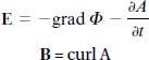
Writing the fields in this form makes certain calculations easier. But in this form we face an underdetermination of the vector potential A by the magnetic field. Since A = A + gradf (for smooth functions of spacetime coordinates, f), it follows that curlA = curl(A + gradf) = B, and so many (formally) distinct vector potentials will represent the same magnetic field (since the curl of a gradient is zero).12 The transformation from one vector potential to another, A → A + gradf, is an example of a gauge transformation, where A is known as the gauge field. Physical quantities will be independent of this field (and dependent only on the magnetic field, or the vector potential ‘up to an arbitrary gradient’; that is, ‘up to a gauge transformation’) and the laws will be covariant with respect to transformations between gauge-related vector potentials. Physical quantities and laws are simply blind to such transformations.
Eugene Wigner describes the introduction of these (seemingly impotent) potentials to represent the states of the electromagnetic field as follows:
In order to describe the interaction of charges with the electromagnetic field, one first introduces new quantities to describe the electromagnetic field, the so-called electromagnetic potentials. From these, the components of the electromagnetic field can be easily calculated, but not conversely. Furthermore, the potentials are not uniquely determined by the field; several potentials (those differing by gradient) give the same field. It follows that the potentials cannot be measurable, and, in fact, only such quantities can be measurable which are invariant under the transformations which are arbitrary in the potential. This invariance is, of course, an artificial one, similar to that which we could obtain by introducing into our equations the location of a ghost. The equations then must be invariant with respect to changes of the coordinate of the ghost. One does not see, in fact, what good the introduction of the coordinate of the ghost does. ([56], p. 22)
When we have a theory with a gauge group, like electromagnetism, we find that our initial (Cauchy) data made at some instant, no matter how complete, will not serve to fix the physical situation if we understand the gauge variables (or frame) to be responsible for representing our physical frame. This distinguishes gauge freedom from the kind of situation we found in the Leibniz shift examples. That also involved an underdetermination of the physical state by the laws, but was not sufficient for indeterminism of the kind found here. Indeterminism, in the gauge theory sense, requires that no amount of specification of initial data can secure unique future values for some physical quantity or object. The gauge transformations can be performed locally, so that we can choose to do it after some initial specification of values has been made. In the case of Newtonian mechanics, there are enough evolution equations to allow us to evolve (or ‘propagate’) all of the physical magnitudes once a labeling of the particles and localizations and velocities have been settled on since the symmetries there are globally defined: once we ‘break’ them, so to speak, everything is fixed thereafter (even if the choice was arbitrary to begin with).13 The indeterminism that lies at the core of gauge theories is an underdetermination of solutions of the equations of motion given an initial data set: no amount of specifying in this sense will enable the laws to develop the data into a unique solution. It is, then, rather a more serious epistemological defect than the absolute velocities in Newton’s theory.
You might wonder why physicists play around with gauge freedom if it’s both damaging and inconsequential. That’s worth wondering about, there’s still much work to be done in fully figuring this out. But we can say that gauge symmetries play a crucial role in identifying the physical content of theories; namely, as that which remains invariant under the gauge transformations. This sounds similar to symmetries, of course, and they are related, but note that gauge symmetries are often referred to as ‘redundancies,’ which indicates a crucial difference. Simply put, symmetries in general are structure-preserving transformations. Usually, symmetries relate one solution of the equations of motion of some theory (or a physical system described by the theory) to another physically distinct solution, albeit in a way that preserves some features (such as the laws or observables). In other words, symmetries are transformations that keep the system’s state within the set of physically possible states. The orbit under the action of a symmetry group consists of points representing distinct situations related by the symmetry transformation. With gauge symmetries, however, though the transformations do still map between physically possible states, they are viewed as representations of one and the same physical state (this protects physical determinism, of course, since there are no physically distinct alternate possibilities). The orbit of the gauge group consists of points that are not just identical in certain physical respects (i.e. in terms of what they represent): they are physically identical, period. In fact, ‘physical state,’ in this context, is really just shorthand for ‘equivalence class of states under gauge symmetries,’ so that physical states are represented by entire gauge orbits rather than their elements.
While symmetries can result in physically distinguishable scenarios, gauge redundancies (as the name suggests) result in no physically observable differences, and so, to get at the ‘real structure,’ are usually removed by a ‘quotienting’ procedure that leaves one with a (reduced) space of orbits of the gauge group. Hence, various representations of a theory’s content can be given, but they will be considered to lie in an equivalence class such that each represents the same physical state of the world. For this reason, Richard Healey adopts the stance that gauge symmetries are cases of ‘multiple realizability’: many ways of realizing some physical state (albeit with redundancy involved in the representation). But the realizations are generated by surplus formal structure (part of the mathematical representation of a theory that should not be given any ontological weight as it stands): “Understood realistically, the [gauge] theory is epistemologically defective, because it postulates a theoretical structure that is not measurable even if the theory is true” ([23], p. 158). As Healey points out, and as we saw above, the natural course of action is to treat the realizations as representations of the same physical situation. Indeed, this ‘mathematical surplus’ approach is the default.
I’m belaboring the point here since one might be led to think that the obvious ontological option in the case of electromagnetism is to commit to the reality of the electric and magnetic fields only: these are what we measure (potentials are unmeasurable), and these are what remain invariant under the gauge transformations (potentials are shifted: gauge-variant). This gauge-invariant interpretation is indeed an obvious choice: we get a one-to-one mapping between the fields and the world (modulo the usual idealizations involved in any physical theory). We simply take the vector potential to be unphysical. However, when we include quantum mechanics the situation appears to radically change, with the vector potential playing a role in the dynamics - the potential figures in the Schrödinger equation and so despite its ‘gaugey’ nature, might need to be given a physical reading. But the problem is that the gauge field is as (directly) unobservable as ever it was: it is determined by the equations of motion only up to the addition of the arbitrary gradient of a function of spacetime.
An experiment devised by Yakir Aharonov and David Bohm (describing the Aharonov-Bohm effect, often just called the ‘AB-effect’) appears to breathe life into the vector potential. The experiment is much like the double slit experiment, only a solenoid (a coil in which a magnetic field can be turned on and off) stands behind the slits. A beam of electrons is fired at a detection screen, and one finds the familiar interference pattern. The novelty is that one can cause the interference pattern to shift (i.e. there is a phase shift), in a predictable way, by turning the current in the solenoid (and so the magnetic field) on and off. That might not strike you as particularly groundbreaking - switching a field on and off is clearly causing it: what’s the problem? The curious aspect is that the magnetic field is zero in the path of the electrons (outside of the solenoid), so this should not be happening. The proposed reality of the vector potential then turns on the fact that this is non-zero in the path of the electrons - due to the fact that integrating the vector potential around a closed loop is equal to the magnetic flux the loop encloses.14
We could stick with the magnetic field as fundamental, but to do so would now involve viewing it as acting-at-a-distance on the electrons. We invoke the potential because we have a desire for local action in physics. However, with the vector potential interpretation we face the problem of underdetermination in which we cannot say which of an infinity of potentials is responsible for the phase shift: the dynamics can only determine the evolution of potentials up to a gauge transformation. Hence, we have to trade local action for indeterminism. How to decide?
Note that the vector potential is still not measured in the experiment (how could it be?), but the loop integral mentioned above (∮A · dx, known as an ‘holonomy’: carrying the vector potential around a loop) is, and this will give the same value for any of the gauge-related potentials: it is gauge-invariant, like the magnetic field. This suggests using such holonomies as an alternative interpretation, which both avoids the problem of action-at-a-distance and the indeterminism/non-measurability: the best of both worlds! The holonomy embodies the invariant structure of the vector potentials since many vector potentials are subsumed in one and the same holonomy: vector potentials give the same holonomies when they are gauge related. However, it is a little hard to see these loopy entities as the stuff of physical reality. Although determinism and local action are restored, another kind of nonlocality re-enters, though of a rather curious kind. The nonlocality concerns the ‘spread outness’ of the variables: they are not localized at points but rather are represented in a ‘space of loops.’15 But must we be committed to this space in an ontological space? If we are so forced, then the problems of action-at-a-distance and indeterminism look rather less bizarre by comparison. But there are always choices that can be made about which parts of a mathematical structure should be mapped to the world.
To sum up: it turns out that there are several distinct ways to formulate gauge theories, each pointing to a distinct interpretation (a different kind of world, with different fundamental furniture), and having distinct virtues and vices. In the electromagnetic case (though it generalizes easily to other gauge theories), you can use local quantities, such as potentials Ai, to represent what’s going on; or you can use nonlocal entities such as magnetic fields; or you can use holistic entities such as the integral of Ai around a path enclosing the region with the magnetic field. The problem with using potentials is that, though they allow a nice local-action account of the Aharonov-Bohm effect, they are ‘unphysical’ variables: not measurable or predictable by the laws. The problem with using magnetic fields is that though they are measurable and predictable, they must act at a distance in order to explain the Aharonov-Bohm effect (well tested and shown to occur). The problem with using holonomies is that, though they are also gauge invariant, they appear ontologically suspect since they are ‘spread out’ (a different kind of nonlocality). Given that this set of options is pretty much generic for gauge theories, it is a pressing task for philosophers of physics to figure out which is to be recommended, or say why the choice doesn’t matter. Crucial to the pros and cons of these interpretive options is the Aharonov-Bohm effect, but it doesn’t necessitate that we believe in the reality of gauge potentials (aka ‘the traditional physicist’s view’).16
What to read next
1. Michael Redhead (2003) The Interpretation of Gauge Symmetry. In K. Brading and E. Castellani, eds., Symmetries in Physics: Philosophical Reflections (pp. 124-39). Cambridge University Press.
2. Gordon Belot (1998) Understanding Electromagnetism. British Journal for the Philosophy of Science 49(4): 531-555.
3. Dean Rickles (2008) Symmetry, Structure, and Spacetime. Elsevier.
Research projects
1. Work out what in your opinion is the best ontology for electromagnetism: fields, potentials, holonomies, or something else. Answer with reference to ‘locality (separability) versus holism (non-separability)’; ‘locality versus action-at-a-distance’; and ‘determinism versus indeterminism.’
2. Should the behavior of the electromagnetic field with quantum particles have any significance for our interpretation of the purely classical theory?
3. Why do we set theories up with gauge freedom? Why not do everything without adding redundant, unphysical elements?
8.4 Quantum Fields
Quantum field theory is the natural home for describing the interaction of charged point particles via the electromagnetic, strong, and weak fields: three of the four forces of nature (gravity not included). In this approach the discrete, particlelike ‘excitations’ (photons, gluons, etc.) of the various (continuous) fields mediate the various interactions - photons, for example, mediate the electromagnetic interaction between charged particles in the context of quantum electrodynamics, providing a nice local account of how such interactions happen. Given that three interactions have succumbed to the quantum field approach, it makes sense to try to accommodate gravity in the same formal framework: here the gravitational interaction would be mediated by the ‘graviton’ (technically: a mass-less, spin-2 quantum particle of the gravitational field). Before we turn to gravity, let us first say something about quantum field theory itself.
As with gauge theories, much of the philosophical work on quantum field theory has tended to focus on what the basic ontology is. We face a difficult problem here, as with gauge theories, since there are many formulations of quantum field theories too, which recommend distinct ontologies. For example, if we use what is called the ‘occupation number’ representation (using Fock space: Hilbert spaces tensor-producted together), then we can make some sense of there being particles (or rather ‘quanta’) in the theory, though, as our earlier discussion of particle statistics implies, they are not quite what we usually mean by particle: though we can say how many we have, they cannot be individually labeled. But, from what we have said above, if there can be physical states with no particles present (the vacuum), then it is hard to view particles as fundamental. There are also problems in upholding a particle picture in other quantum field theoretic contexts, such as curved spaces in which the notion of particle is seemingly impossible to establish (in the absence of the symmetries supplied by the usual spacetime metric) - to speak of particle number as an observable quantity requires that there be a particle number operator, but this seems to be specific to flat, Minkowski spacetime.
A field approach (i.e. in which fields are the basic entities in the world) is the natural alternative to a particle interpretation. But there are issues here too. Not least the problem of mapping quantum fields to the world. Particles can at least be directly associated with objects in the world, but fields in a quantum theory are operator-valued, so we have an inherent indirectness in the mapping. Attempts have been made to reconnect fields and world by employing expectation values of the field instead, which provides a numerical value. But such approaches still involve an indirectness since ‘expectation’ is a statistical concept invoking the average value given many measurements. Moreover, in most practical applications of quantum field theory it is the particles that are center stage - in scattering experiments at CERN, for example.17
Note that these ontological considerations go deeper than the usual interpretative options for quantum mechanics (many worlds, Copenhagen, etc.): whatever basic ontology we settle on will then face this next level of interpretation. Likewise, if we find that the world is described by quantum strings or branes, then these too will face the usual interpretive suspects for quantum theories.
Ordinary quantum mechanics and quantum field theory are brought closer together if the wavefunction is considered the primary thing. In the case of quantum field theory this is more properly a wavefunctional, or a function that takes another function (in this case the field associating field values to spacetime points) to some number (the probability for finding some classical field configuration). The usual measurement problem arises given this wavefunctional approach since we can have superpositions of classical field configurations (just as we could have superpositions of, e.g. spin states of a single particle). This also faces problems. Again, it’s hard to square with the apparent ‘practical primacy’ of particles. Moreover, the interpretive problems associated with the measurement problem take center stage. And, perhaps worse, the wavefunctional is hard to make sense of given that it maps entities defined on spacetime, but itself is defined with respect to a very complicated field-configuration space.18
There are very many more philosophically interesting issues facing quantum field theory. To delve into these would require too much by way of preparation.19 Instead, let us simply focus on one aspect that stems from the relative treatments of vacuum in quantum field theory and general relativity, and then segue into a discussion of quantum gravity, which involves an apparent failure of the usual techniques of quantum field theory when applied to gravity. Many of the problems have to do with the treatment of space and time in the two contexts.
For example, in the good old days ‘vacuum’ meant complete emptiness: no energy, no matter, no particles, no fields. Just pristine empty space. Both quantum field theory and general relativity spoil this clean division into empty space and matter. In our discussion of the hole argument, we saw how space becomes more ‘matterlike’ in general relativity, obeying its own equations of motion, allowing ‘ripples of spacetime’ (gravitational wave solutions) to be used to do work. Mixing quantum mechanics and special relativity (to give quantum field theory) spoils things in a different way since the vacuum state is no longer a state with zero energy, but merely a state with the ‘lowest’ (non-zero) energy. As such it is distinguished in being the ground state, but not really so different from non-vacuum states ontologically speaking.
This framework leads to a serious conflict between general relativity and quantum theory known as the ‘cosmological constant problem.’ The energy spectrum for an harmonic oscillator, EN = (N + 1/2)ω, has a non-vanishing ground state in quantum mechanics (the ‘zero-point energy’) resulting from the uncertainty principle (so that it is impossible to fully ‘freeze’ a particle so that it has no motion at all, no oscillations). In quantum field theory the field is viewed as an infinite family of these harmonic oscillators (one at each point of space, and each with a little bit of zero point energy), so that the total energy density of the quantum vacuum must be infinite. Of course, general relativity couples spacetime geometry to energy, but if this energy is infinite in any spacetime region then that region will have an infinite curvature. But it clearly doesn’t: so what is wrong?
There are ways to tame this infinity. For example, just as there is no absolute voltage in classical electromagnetism (because there is no zero point, only potential differences between points), so one can say the same about the quantum vacuum. If only energy differences between the vacuum and energy states make any sense we can simply rescale the energy of the vacuum down to zero. The absolute value of the energy density of the quantum vacuum is unobservable; the value one gives is largely a matter of convention.20
But, the clash between general relativity and quantum field theory strikes back since this rescaling is not possible in cosmology. The cosmological constant, or vacuum energy, is taken to just be a measure of the energy density of empty space. This allows an experimental approach to be adopted to determine the correct value using general relativity’s link between mass-energy and spacetime curvature. The energy density ρ, as actually observed in curvature measurements, comes out at around 10−30g cm−3: very close to zero, which is a long way from the naive (enormous) expectations suggested by quantum field theory - that is, once we perform various other infinity-taming procedures, that we needn’t go into here. Resolving this problem is one of the challenges for a quantum theory of gravity. A straightforward application of the usual rules of quantum field theory does not work with gravity - though it has taken many decades of struggle to figure this out.21
This is just one example of the conflict between our two best theories of the universe, general relativity and quantum field theory. There are others, most often stemming from the different ways space and time are treated in these frameworks: in quantum field theories, space and time function as fixed structures, seemingly essential for making sense of the core components of the theory (the inner product, the symmetries, the probability interpretation, etc.); in general relativity, spacetime is a dynamical entity.
As in the other examples of quantum field theories (especially for the strong interaction, which has certain important features in common with gravity), quantum gravity along these lines runs into formal difficulties: when one tries to compute probability amplitudes for processes involving graviton exchange (and, indeed, involving the exchange of other particles in quantum field theory) we get infinities out. Since we cannot readily make sense of measuring infinite quantities, something has clearly gone wrong. In standard quantum field theories, quantum electrodynamics for example, these infinities can be ‘absorbed’ in a procedure called renormalization (similar to the rescaling of the zero point energy as mentioned above). The problems occur when the region that is being integrated over involves extremely short distances (or, equivalently, very high momenta, and so energies, for the ‘virtual particles’).22 In quantum gravity, as the momenta increase (or the distances decrease) the strength of the interactions grow without limit, so that the divergences get progressively worse - the problem is: gravity gravitates, so that the gravitons will interact with other gravitons (including themselves!). The usual trick, in quantum field theory, of calculating physical quantities (that one might measure in experiments) by expanding them as power series (in the coupling constant giving the interaction’s strength) fails in this case, since the early terms in such a series will not provide a good approximation to the whole series.
This gives us one way of understanding quantum gravity: a microtheory of gravity. Or, since gravity is understood via the geometry of spacetime, the microstructure of spacetime geometry. (Hence, quantum gravity is often understood as a theory of quantum spacetime. But there are approaches that do not involve quantum properties of the gravitational field (and so spacetime); they do not quantize gravity at all, but might, for example, have gravity (and spacetime) emerge in a classical limit.) At large scales we know general relativity works well, but it buckles at short distances (with singularities being one symptom of this). The scales at which infinities appear like this signal the limit of applicability of general relativity, and point to the need for a quantum theory of gravity (or some other theory that can reproduce the predictions of general relativity at those scales in which it does work - superstring theory is an example of this approach). In other words, the picture of a smooth spacetime that we are used to in physics might fail at a certain energy. (This limit of applicability of the general theory of relativity is known as the Planck scale. Quantum gravity is, for this reason, also sometimes understood as whatever physics eventually describes the world at the Planck scale.) This in itself points to a more skeptical attitude towards the techniques of (orthodox) quantum field theory since they assume a spacetime that is smooth and continuous ‘all the way down.’ There are recent approaches that distance themselves from this assumption, either putting discreteness in as a basic postulate (as in ‘causal set theory’) or else deriving discreteness as a consequence of the theory (as in ‘loop quantum gravity’).23 Without the assumption of smoothness, many of the divergence (i.e. infinity) problems evaporate since there is an end point to the scales one can probe (that is, there is a smallest length, area, and volume).24
Much of the discussion, philosophical and technical, tends to deal with free quantum fields, in which interactions are ‘turned off.’ Dealing with interactions is notoriously difficult and, indeed, faces something known as ‘Haag’s Theorem,’ which indicates that interacting quantum field theory cannot be established within a consistent mathematical framework. This is suggestive of the difficulty of quantum field theory, which is justified in many ways. To discuss its conceptual issues properly requires deep and lengthy investigation: there’s no way around it. I can do no better than to point readers at the beginning of this journey to Paul Teller’s book in the ‘What to read next’ section below.
What to read next
1. Paul Teller (1995) An Interpretive Introduction to Quantum Field Theory. Princeton: Princeton University Press.
2. Sunny Auyang (1995) How is Quantum Field Theory Possible? Oxford University Press.
3. Meinard Kuhlmann, Holger Lyre, and Andrew Wayne, eds. (2002) Ontological Aspects of Quantum Field Theory. World Scientific Pub Co Inc.
Research projects
1. Is quantum field theory, fundamentally, a theory of particles or fields (or neither)?
2. What exactly is it about curved spacetime that causes problems for a particle interpretation of quantum theory? Can particles be included at all in such curved backgrounds? Where does this leave particles in a quantum theory of general relativity?
3. Describe and evaluate wavefunction realism in the context of quantum field theory.
8.5 Frozen Time in Quantum Gravity
There are very many points of contact between physics and philosophy in the case of quantum gravity. Here, to keep the length manageable, we focus on an issue that has received the most attention from philosophers, achieving a degree of notoriety: the problem of time - it helps that this has much in common with the hole argument discussed in §4.4.
The response to the hole argument according to which diffeomorphism invariance points to gauge freedom in the theory (understood relationally or otherwise), so that diffeomorphisms do not correspond to physical changes, has some curious consequences: since time evolution is an example of such a diffeomorphism transformation (e.g. mapping some point (1,0,0,0) into (0,0,0,0)), the observables of the theory - the gauge-invariant (diffeomorphism-invariant) content - are insensitive to such changes. Indeed, the ‘temporal’ evolution takes place along a gauge orbit so understood since each temporal diffeomorphism counts as a gauge transformation. But surely a theory’s observables are the kinds of thing that change over time, from one instant to the next? If not, then general relativity appears to be frozen, with observables that look the same on each time slice through the spacetime. This doesn’t correspond to our experimental and experiential life, so mustn’t we reject the theory?
Note that there is an interesting link to relationalist and substantivalist conceptions of spacetime here. According to the logic of Earman and Norton’s presentation of the hole argument, the latter will view each of the temporal advances as generating physically distinct scenarios (since the observables are located on different time slices in each case), but there will nonetheless be no observable change: all invariants are preserved, just as the formally distinct futures in the hole argument preserved invariants (and observable content). Thus, the substantivalist faces the problem of the hole argument in this temporal case: possibilities that differ only in which points (now characterizing a time slice) play which role. But the relationalist’s standard Leibnizian trick of collapsing all the substantivalist’s indiscernible possibilities into one physical possibility doesn’t help us here, since it leaves us with data on a single three-dimensional slice. Any attempt to push the data forward will generate an unphysical possibility, so we appear to be stuck on this slice, unable to generate change! It doesn’t matter whether we are substantivalists or relationalists here: there will be no change in observables if those observables are defined relative to spacetime (manifold) points.
The problem takes on its clearest form in the canonical formulation of general relativity, in which the dynamics (time evolution) of the geometry of space is generated by a Hamiltonian function: we find that it vanishes (as is expected given its gaugey nature: it can’t push the data forward in a non-unphysical way). Being a gauge theory, the Hamiltonian is really to be understood as a family of constraints: three spatial (or ‘diffeomorphism’ or ‘vector’) constraints and a temporal one (known officially as the ‘Hamiltonian’ or ‘scalar’ constraint). We can think of the spatial constraints as simply transformations that bring about ordinary coordinate changes on a spatial slice (the kind found in the hole argument). These can be dealt with in the usual ‘equivalence class’ manner: the transformations are unphysical → the physical stuff is the equivalence class → all is well. The Hamiltonian constraint generates displacements of data off the spatial slice. The overall Hamiltonian, responsible for generating the time evolution of states in the theory, is simply a linear combination of these two kinds of constraint. Taken together, they generate (infinitesimal) spacetime diffeomorphisms - this explains why physical observables (sometimes called ‘Dirac observables’) can’t evolve with respect to the Hamiltonian, since such observables are gauge-invariant entities and diffeomorphisms are gauge transformations.
This problem infects quantum gravity in a fairly direct way: since the Hamiltonian and the observables are quantized by turning them into operators (and imposing commutation conditions), the problem sticks around.25 But it takes an even worse form: whereas the Schrödinger equation usually involves a t against which quantum states evolve (i.e. as ![]() , we have a truly timeless theory now: the t doesn’t even make an appearance in the theory since the classical Hamiltonian, to be quantized and converted into the Schrödinger equation (or rather its gravitational analogue, ‘the Wheeler-DeWitt equation’), vanishes:
, we have a truly timeless theory now: the t doesn’t even make an appearance in the theory since the classical Hamiltonian, to be quantized and converted into the Schrödinger equation (or rather its gravitational analogue, ‘the Wheeler-DeWitt equation’), vanishes: ![]() . It is a sum of constraints (on initial data) rather than a true dynamical equation. But without a time, how do things change and evolve? How is there motion?
. It is a sum of constraints (on initial data) rather than a true dynamical equation. But without a time, how do things change and evolve? How is there motion?
We can choose to deal with this problem at either the classical (prequantization) level or the quantum level. In either case, we have two broad options: either find a time buried in the formalism or else bite the bullet (that reality is timeless and changeless), leaving the task of explaining away the appearance of time and change in the world (as a kind of illusion). The physicist Karel Kuchar˘ suggested the terminology of ‘Parmenidean’ and ‘Heraclitean’ to describe these fundamentally ‘time-full’ and ‘timeless’ responses.
Kuchar˘ himself is Heraclitean, and sees as the only way out of the frozen formalism (and the quantum version) a conceptual distinction between the constraints so that only the diffeomorphism (spatial) constraints are to be viewed as generators of gauge transformations. This leaves the problem of finding a hidden ‘internal’ time (and so a physical, genuine Hamiltonian) buried among the phase space variables against which real observable change happens. This is a difficult issue that we can’t go into here, but we can point out that some responses along these use the distribution of matter to ‘fix’ some coordinate system, eliminating the gauge symmetry in the process. The usage of physical degrees of freedom to resolve the problem is, in general, the most promising way to go.
Perhaps the most philosophically shocking approach is Julian Barbour’s Parmenidean proposal. Barbour argues that we should accept the frozen formalism: time really doesn’t exist! What exists is a space of Nows (spatial, three-dimensional geometries) that he calls ‘Platonia.’ In the context of quantum gravity we would then have a probability distribution over this configuration space (as determined by the Hamiltonian constraint or Wheeler-DeWitt equation) that delivers an amplitude for each possible Now - where each three-geometry is taken to correspond to a ‘possible instant of experienced time.’
But unlike the Heraclitean proposals, which strive to get out real change (and so can account for our experience of a changing world), on Parmenidean proposals there remains the problem of accounting for the appearance of change. Barbour attempts to resolve this puzzle by appealing to what he calls ‘time capsules,’ patterns that encode an appearance of the motion, change, or history of a system - he conjectures that the probability distribution determined by the Wheeler-DeWitt equation is peaked on time capsules, making their realization more probable (this makes it more likely we will experience a world that looks as though it has evolved through time, and so has generated a history, or a past).
Barbour’s approach is certainly timeless in that it contains no background temporal metric in either the classical or quantum theory: the metric is defined by the dynamics. His view looks a little like presentism - the view that only presently existing things actually exist - but clearly differs since there are a bunch of other Nows that exist, only not in the same spacetime (but ‘timelessly’ in ‘superspace’ instead). This space of Nows might in fact be employed to ground a reduction of time in the same way David Lewis’ ‘plurality of worlds’ provides a reduction of modal notions.26 The space of Nows is given once and for all and does not alter, nor does the quantum state function defined over this space, and therefore the probability distribution is fixed too. But just as modality lives on in the structure of Lewis’ plurality, so time can be taken to live on in the structure of Platonia.
The jury is still out on the coherence of Barbour’s vision (philosophical and otherwise), but it makes a fun and worthwhile case study for philosophers of physics who like to think about time, change, and persistence. Not quite as radical as Barbour’s are those timeless views that accept the fundamental timelessness of general relativity and quantum gravity that follows from the gauge-invariant conception of observables, but attempt to introduce a thin notion of time and change into this picture - these fall uncomfortably between the Heraclitean and Parmenidean notions.
A standard approach along these lines is to account for time and change in terms of time-independent correlations between gauge-dependent quantities. The idea is that one never measures a gauge-dependent quantity, such as position of a particle; rather, one measures ‘position at a time,’ where the time is defined by some physical clock. Carlo Rovelli’s ‘evolving constants of motion’ proposal is made within the framework of a gauge-invariant interpretation. As the oxymoronic name suggests, Rovelli accepts the conclusion that quantum gravity describes a fundamentally timeless reality (so that there are only unchanging, time-invariant, constants of motion), but argues that sense can be made of change within such a framework by ‘stringing them together.’ Take as a simplified example of an observable m = ‘the mass of the rocket.’ As it stands, this cannot be a genuine (gauge-invariant) observable of the theory since it changes over (coordinate) time (it does not take on the same value on each time slice since it will be losing fuel as it travels, for example). Rovelli’s idea is to construct a one-parameter family of observables (constants of the motion) that can represent the sorts of changing magnitudes we observe. Again simplifying, instead of speaking of, e.g. ‘the mass of the rocket’ or ‘the mass of the rocket at t,’ which are both gauge-dependent quantities (unless t is physically defined: i.e. the hand of an actual clock), we should speak of ‘the mass of the rocket when it entered the asteroid belt,’ m(0), ‘the mass of the rocket when it reached Mars,’ m(1), ‘the mass of the rocket when it reached the human colony,’ m(2), and so on up until m(n). These quantities are each gauge invariant (taking the same value in any system of coordinates), and, hence, are constants of the motion. But, by stitching them together in the right way, we can explain the appearance of change in a property of the rocket (understood as a persisting individual). The obstacles to making sense of this proposal are primarily technical, but philosophically we can probe the fate of persisting individuals given such a view, among other issues of perennial interest to philosophers.
A large portion of the philosophical debate on the problem of time tends to view it as a result of eradicating indeterminism via the ‘quotienting procedure’ for dealing with gauge freedom - as mentioned in the previous section, and as found in the hole argument literature: treating the physical structure as encoded in a reduced space involving as points the equivalence classes of gauge-related states. This point of view can be seen quite clearly in a 2002 debate between John Earman and Tim Maudlin,27 where both authors see the restoration of determinism via hole argument type considerations as playing a vital role in generating the problem - but whereas Earman sees the problem as something that needs to be accepted and explained, Maudlin views the problem as an indication of a pathology in the (Hamiltonian) formalism that generated it.
The idea is that when the quotienting process is performed in a theory in which motion corresponds to a gauge transformation, time is thereby eliminated. But the world is frozen regardless so long as we deal with physical observables (those that are insensitive to the gauge-changes brought about by the constraints, and so the Hamiltonian). Hence, we could forget the quotienting, and let time merrily advance, but nothing observable will register this difference.
Earman and Maudlin couch their debate in terms of an argument against the existence of time due John McTaggart. In a classic 1908 paper, “The Unreality of Time,” McTaggart argued that we can think of positions in time in two ways: first, each position is earlier than some and later than others (known as the B-series); and secondly, each position is either past, present, or future relative to the present moment (known as the A-series). The first involves a permanent ordering of events, while the second does not: if an event E1 is ever earlier than event E2, it is always earlier. But an event, which is now present, was future, and will be past. We met this kind of alteration in the ontological status of events (under the umbrella of ‘becoming’) in §4.3. This corresponds to the ‘flow of time’ (common to our experience of the world), consisting of later events becoming present and then past: time passes in this way. McTaggart had argued that both series are needed to account for time. To make sense of flow, we can think either of sliding the B-series ‘backwards’ over a fixed A-series or sliding the A-series ‘forwards’ over a fixed B-series.
The B-series is seen to depend on the A-series since the only way that events can change is with respect to their A-properties, not their B-relations (which are eternally fixed): the event ‘the death of Alan Turing’ does not change in and of itself, but, given the A-series, it changes by becoming ‘ever more past,’ having been future, relative to the Now. So ‘Alan Turing is dead’ changes its truth-value: during all of those B-series positions in which Turing is alive (or not yet born) the proposition is not true, but is true thereafter. But B-series versions do not have this time-varying feature: ‘Alan Turing’s death is earlier than this judgment’ is either always true or always false. But this ordering isn’t enough for time since there is no change.
So McTaggart concludes that time needs an A-series to ground the notion of change. But then he argues that the A-series, and therefore time, is contradictory. A-properties (‘is past,’ ‘is present,’ and ‘is future’) are mutually exclusive (they conflict), but events must posses all of them: a single event like ‘Turing’s death’ is present, will be past, and has been future. The problem looks like it can be evaded by pointing out that no event has all three properties ‘at the same time’ (simultaneously), but this leads to a regress: is present, will be past, and has been future all involve some additional ‘meta-moments,’ which will also face the problem of being all of past, present, and future - the obvious save now is to invoke ‘meta-meta-moments,’ and we are on the road to an infinity of such meta-levels. So McTaggart claims that time does not exist: the B-series can’t cope with the demands of time on its own and the A-series, which it requires, is incoherent.
So much for the A- and B-series: what is left to put in their place? McTaggart suggests that an ordering of events remains, a C-series, but this cannot be temporal, for it does not involve change, being a serial ordering of events themselves - that we have a string of events, E1, E2, E3, implies that there is any change no more than the ordering of the letters of the alphabet implies change. Modern philosophers of time are divided over whether an A-series (or something similar) in needed to make sense of time and change: the nay-sayers are grouped into the category of B-theorists or ‘detensers’ and the yea-sayers are grouped into the category of A-theorists or ‘tensers.’ The A-theorists will say that the B-theorists cannot properly accommodate the notion of the passage of time and can, at best, allow that it is an illusion. The B-theorist denies that ‘passage’ is necessary for time and change, and is happy to see it done away with. Both sides claim support from physics: B-theorists generally wield spacetime theories (such as special relativity) and the A-theorists wield mechanical theories such as quantum mechanics.
What is interesting about the problem of time in quantum gravity is that neither the A- nor the B-series seems to make sense anymore. To link up these old-fashioned philosophical concepts to quantum gravity, Earman introduces a character called ‘Modern McTaggart,’ who attempts to revive the conclusions of old McTaggart by utilizing a gauge-theoretic interpretation of general relativity. Earman is dismissive of A-theories, which he claims are not part of “the scientific image.” But it is important to note that the debate here is not directly connected to the old debate in the philosophy of time between ‘A-theorists’ and ‘B-theorists’ (or ‘tensers’ and ‘detensers’). Both of these latter camps agree that time exists in a sense (they are committed to some t in the physical world), but disagree as to its nature. By contrast, the division between Parmenidean and Heraclitean interpretations concerns whether or not time (at a fundamental level) exists, period!
Earman’s response is to argue that general relativity is nonetheless compatible with change, though in neither the B- nor the A-series (nor the C-series) senses. Instead he introduces a ‘D-series’ ontology consisting of a time-ordered sequence of ‘occurrences’ or ‘events’ in which different occurrences or events simply occupy different positions in the series. This sounds like the C-series, but the occurrences here are the gauge-invariant quantities involving relationships between physical degrees of freedom (like Rovelli’s evolving constants of motion, which Earman’s strategy gives a philosophical expression of). There is no flow here, but there is change embedded in the different events laid out in different D-series positions. The only difference between the C-series and the D-series then is in the nature of the events that are strung together. In the case of a D-series picture one of the elements of a gauge-invariant quantity can be a physical clock (a wristwatch), against which is considered some other element (such as your position relative to your front door) so that we can see how something mirroring experience might be elicited from this picture. But strictly speaking, nothing is changing here.
For Maudlin, any such interpretation is absurd. The absence of change should be a reason to reject whatever framework led to that conclusion. Maudlin sees the problem to be taking a ‘surface reading’ of general relativity too literally, where such a reading cannot explain why a bizarre frozen-world conclusion is emerging. But, as we have seen, it can explain the changelessness and the appearance of change. The answer is related to the gauge-invariant response to the hole argument: change with respect to the manifold is ruled out; if we focus on those quantities that are independent of the manifold we can restore change by considering the ‘evolving’ relationships between these quantities. That is: change is to be found in things other than the manifold, namely in the relationships between physical degrees of freedom. That is, the crazy sounding results only come about by considering the wrong types of observable: gauge-dependent, unphysical ones. But this is to adopt a substantive response that buys into the gauge-theoretical interpretation!
Finally, if we agree with the Parmenideans that we don’t have space and time at the level of quantum gravity, then where does the classical spacetime we appear to be immersed in come from? This leads to the problem of ‘spacetime emergence.’ In other words, saying that quantum gravity is timeless (and spaceless) leaves a challenge in squaring it with the low-energy physics that appears to involve such entities - not to mention the evidence of our senses. This is a difficult problem, but steps have been taken in doing exactly this.
In the author’s view, quantum gravity offers the biggest open problem for philosophers of physics and it really ought to be a bread and butter topic: it is, with its novel views on time, change, space, persistence, and so on, a playground for philosophers.
What to read next
1. Craig Callender and Nick Huggett, eds. (2001) Physics Meets Philosophy at the Planck Scale. Cambridge University Press.
2. Jeremy Butterfield and Chris Isham (1999) On the Emergence of Time in Quantum Gravity. In J. Butterfield, ed., The Arguments of Time (pp. 111-168). Oxford University Press.
3. Dean Rickles (2008) Quantum Gravity: A Primer for Philosophers. In D. Rickles, ed., The Ashgate Companion to Contemporary Philosophy of Physics (pp. 262-382). Ashgate.
Research projects
1. Consider which (if any) philosophical account of persistence (of individuals) fits with Rovelli’s evolving constants of motion approach.
2. Read Julian Barbour’s book The End of Time (Oxford University Press, 2001) and decide whether his theory is really timeless.
3. Figure out whose side you’re on (if any) in the debate between Tim Maudlin and John Earman over the use and interpretation of the constrained Hamiltonian formalism in general relativity.
8.6 Fact, Fiction, and Finance
Physics is powerful. It is often seen to be a universal science, providing the ontological roots of all of the other sciences. But just how powerful? Where does the domain of physics end and, say, the social sciences or psychology begin? Of course, most of us wouldn’t hesitate in agreeing that any social system and human mind are essentially ‘built from’ components obeying physical laws: if they violated the laws of physics then so much the worse for those systems and minds. These days at least, the ‘physics versus everything else’ separation is attributed to the complexity of the systems, sometimes with a nod to a future in which physics can crack the problems of society and consciousness too: such features (including ‘higher-level laws’) will be ‘emergent’ properties of the physical systems realizing them.28
If we agree that economic systems are complex systems, then a natural policy for a physicist is to try to adapt the techniques of statistical physics (the complex system theory par excellence) to the description and prediction of economic phenomena. ‘Econophysics’ then describes a cluster of methods and models designed to capture the (statistical) properties and behavior of economic systems (usually just restricted to financial markets) using theories of physics (primarily statistical physics).29 It sits, in terms of disciplines, more in physics than economics (a social science), and one can now find econophysics papers appearing in physics journals, side by side with papers on dark matter and quark-gluon plasmas.
But the simple ‘econophysics = statistical physics of finance’ link is an approximation. We can in fact discern several layers to this proposed physics-economics link:
· Econophysics involves a kind of statistical mechanics of financial markets.
· Econophysics is a proper empirical study of financial data: a data-first approach (rather than model-first), in which economic assumptions are not made at the outset.
· Econophysics involves viewing financial/economic systems as complex systems with interacting economic agents as parts.
· Econophysics is the general application of the models, theories, and concepts of physics (not just statistical physics) to financial markets.
· Econophysics is the idea that financial markets (and economic systems more generally) follow similar laws (or the same kind of laws) as ‘natural’ systems.
· Econophysics involves finding analogies between financial/socioeconomic and physical (natural) systems.
The motivation behind each separate conception is the potential for prediction (and control) and explanation of some market quantities (price, volume, or volatility of some ‘financial instrument’) or events (notably, bubbles and crashes - i.e. large fluctuations or ‘extreme’ events - and more general market trends), through the formulation either of equations of motion derived, in this case, through the recognition of patterns and signatures in the data or the formulation of statistical laws that the quantities or events obey. How does this look in practice? At the core is a postulated mapping between a general model from physics (a model of cooperative phenomena) and the behaviors of economic agents - note that “cooperative” in this context does not mean the nice, social idea of working together for the greater good, but simply the degree of imitation involved among a system’s parts.
The global financial crisis that began around 2007 is commonly believed to be traceable to the relative ease with which borrowing for home loans could be done before that time - fueled by the widespread belief that property was as ‘safe as houses’ and so allowing for the creation of ‘subprime mortgages’ given to those with low credit ratings (i.e. not enough money to handle dips in the value of whatever the loan was for, or rises in external living values). But the banks weren’t stupid (just highly unethical!): they charged more (in interest) to those able to afford less, in order to cover their own increased risk. This led to a boom in house buying, with prices increasing and the expectation that they would continue to increase - some used the value stored in their existing homes to fund other homes. But such a situation is naturally very fragile to ‘shocks.’ The complexity features come from this aspect: there is an interdependency between the various economic agents in that they require that the prices keep going up (with low interest rates) so that they can keep up with their payments - seeing buying occurring brings in yet more buyers (driving the prices up) troubled by the ‘fear of missing out’ (FOMO: which results in a kind of human-herding behavior). This naturally leads to a greater chance of slipping behind in mortgage payments and ultimately ‘defaulting’ on their loan (losing their home) if anything should alter the rising price trajectory - even small dips could result in significant losses of property for those with subprime mortgages. As soon as the foreclosures start, supply increases, and prices reduce, causing more selling in a bid to avoid large losses, which triggers more selling at a faster rate (driving prices down) - and so on in a snowball effect until the financial equivalent of an avalanche occurs.
Hence, we have the economic notions of boom and bust, or bubbles and crashes. This can be linked quite naturally to aspects of cooperative phenomena in statistical physics. The trick involves viewing economic agents along the lines of a ‘spin model’ of ferromagnetism. Each agent has a set of states that they can occupy, switching between them according to certain intrinsic properties (e.g. such as how risk-averse they are), but also, crucially, able to become dependent on the structural properties of the economic system as a whole by ‘nearest neighbor interactions,’ which can spread over a system in certain contexts. Hence, just as magnetism occurs when the spins of atoms in the material point in the same way (demagnetizing otherwise, when they point in random directions), so economic agents can ‘point the same way’ (all buying or all selling at the same time, thus generating bubbles and crashes). In the case of magnetism one needs a parameter, such as temperature, that can be tuned to generate the cooperative behavior of the atoms: heating causes randomness, but cooling causes an orderly structure to emerge. In between these two phases (order and disorder) is a ‘critical point’ relative to the tuning of the parameter, characterized by very specific statistical properties involving events of all sizes distributed according to a power law (roughly: many small events, not so many mid-sized events, and very few large events, as with the distribution of earthquake magnitudes). Such distributions signify complexity in the system, with parts heavily interdependent.
Economic bubbles are then modeled as systems in a critical phase. The cooperative tendency here is simply the herding instinct as above and is modeled by long-range correlations that spread over the system. In such critical, highly cooperative scenarios even tiny shocks to the system can trigger calamitous effects, such as crashes (i.e. spontaneous switches to some value). In these cases it doesn’t make sense to say that some individual event caused the crash: the system was led into an unstable state over time by internal processes. Crashes are systemic (endogenous) making ‘causal postmortems’ very difficult.
The most common model of this type is the Ising model. This models the cooperative coupling between elements by a parameter K, and the tendency to disorder by a noise term (or rather its amplitude) σ. There will be order if K dominates and disorder if σ dominates. Crucial is the existence of a ‘critical value’ Kc of K, which separates these phases: when K < Kc there is disorder and little cooperation or herding (because the elements are effectively disconnected there is no threat of bubble-type behavior emerging). As K tends toward Kc clusters of order form, in which the elements are aligning their values in such a way that alignment in one region can spread, causing alignment in other areas, meaning that the elements are now interconnected. This means that a small shock, which would otherwise be insignificant, can cause an entire system to shift. At the critical point one finds that the system is ‘scale invariant’ in the sense that zooming in and out one finds the same statistical features (relative to the temporal or spatial resolution): it is a fractal. The interconnectedness is, according to econophysics, behind the crashes: they are collective effects or emergent features. Poised at a critical point Kc (in which there is symmetry in the possible states), small influences can break the symmetry (corresponding to K > Kc) and self-organization occurs.
There are other aspects that suggest a statistical physics approach, and that are similarly described. In financial economics there is a group of features known as ‘stylized facts,’ which are properties that are common across many financial objects (stocks, bonds, etc.), markets (money, gold, property etc.), and time periods. For example, prices and their changes appear to be random; returns appear not to be random since their statistical distributions possess so-called ‘fat tails’ associated with the power-laws mentioned above (showing a greater likelihood for extreme values than a simple random, Gaussian distribution would allow); and finally, volatility (fluctuations) is not uniformly distributed, but clusters so that there are highly volatile and non-volatile periods (big price changes, of either sign, follow big price changes and little ones, of either sign, follow little ones). This suggests that the standard model of economics (based on the randomness assumption) is not mapping onto economic reality: stock market crashes of the magnitude of, say, the 1929 Wall Street or 1987 (‘Black Monday’) crashes, should not be occurring as often as they do. Econophysicists claim to be closer to reality in this respect.
Very often in systems with interacting parts, and whose interacting parts generate properties of the unit system, one finds that the thus generated properties obey scaling laws. Scaling laws tell us about statistical relationships in a system that are invariant with respect to transformations of scale. In statistical physics these scaling laws are viewed as emergent properties generated by the interactions of the microscopic subunits. Scaling laws are explained, then, via collective behavior among a large number of mutually interacting components. The components in this financial case would simply be the market’s ‘agents’ (traders, speculators, hedgers, etc.). These laws are ‘universal laws,’ independent of microscopic details, and dependent on just a few macroscopic parameters (e.g. symmetries and spatial dimensions). Econophysicists surmise that since economic systems consist of large numbers of interacting parts too, perhaps scaling theory can be applied to financial markets; perhaps the stylized facts can be represented by the universal laws arising in scaling theory. This analogy is the motivation behind a considerable chunk of work in econophysics; it is through this analogy, then, that the stylized facts receive their explanation - though presumably not their ‘ultimate explanation,’ which will involve such things as the agents’ psychology, the institutions in which the agents operate, and so on.
This ‘scaling’ (or scale invariance) is, then, at the root of the transference of statistical physics to finance. Notably, from the point of view of complexity research, the power law distributions are scale invariant (like fractals): events (or phenomena) of all magnitudes can occur, with no characteristic scale. What this means is that the (relative) probability of observing an event of magnitude |x| = 1,000 and observing one of |x′| = 100 does not depend on the standard of measurement (i.e. on the reference units). The ratio between these probabilities will be the same as that for |x| = 1,000 and |x″| = 10,000. Hence, there is no fundamental difference between extreme events and events of small magnitude: they are described by the same law. Specifically: near a critical point, fluctuations of the (macroscopic) order parameter will appear at all possible scales. In the case of the more common liquid-gas phase transition one will have liquid drops and gas bubbles ranging from the molecular level to the volume of the entire system. Hence, at the critical point these fluctuations become (theoretically) infinite. The analogous situation in the financial context would be, for example, fluctuations in asset returns at all possible scales.30
What distinguishes econophysics from other approaches in economics is the interpretation of the stylized facts. In addition to viewing them as emergent properties of a complex system, it also includes a greater commitment to the stylized facts, treating them not only as a central guide to the nature of economic reality, but also as genuine laws rather than ‘mere’ local regularities. Part and parcel of this view of the stylized facts as genuine laws is that it simply doesn’t matter whether we view the variables of a statistical physics model as spins of atoms or economic agents since the laws themselves are emergent in precisely the sense that they don’t depend on the microscopic details of the system.
However, this stance is, on the face of it, rather hard to square with the addition of decision-making agents (with free will): such agents are surely incompatible with the possibility of invariances, and without invariances there are no symmetries, and without symmetries there are no laws. We might think that, on this basis, like economics, econophysics can at best be a descriptive historical science, analyzing what already happened in some particular economic situation. Other econophysicists (most, in fact) believe that they can find some laws for market dynamics, albeit statistical ones, of course. But, it might be objected, whereas laws of nature are independent of initial conditions and don’t make reference to specific, particular systems, socioeconomic laws seem not to be of this sort, varying from country to country and institution to institution: markets just embody what economic agents do, and since these agents have free will, they can change at a whim. This could affect the more general statistical laws too since the distributions are determined by the collective behavior of the economic agents. But the econophysics argument insists that these collective properties and laws are sufficiently robust that they can ignore the human nature of the agents.31 After all, if humans are not viewed as supernatural ‘magical beings’ then they must surely be governed by physical law. The proof is no doubt in the pudding, and we must await the construction of statistical models that enable reliable predictions about (distributions of) financial properties and their fluctuations. Moreover, a thorough analysis must proceed by carefully unpacking exactly what is meant by ‘law,’ ‘free will,’ and the other central (and difficult) concepts relevant to the debate - in other words: lots of interesting work for philosophy!
What to read next
1. Didier Sornette (2003) Why Stock Markets Crash: Critical Events in Complex Financial Systems. Princeton University Press.
2. Neil Johnson et al. (2003) Financial Market Complexity: What Physicists can tell us about Market Behavior. Oxford University Press.
3. Dean Rickles (2011) Econophysics and the Complexity Of Financial Markets. In C. Hooker, ed., Handbook of the Philosophy of Science. Volume 10: Philosophy of Complex Systems (pp. 531-565). Elsevier.
Research projects
1. Can econophysical models really be said to explain economic phenomena?
2. Are ‘stylized facts’ examples of emergent properties?
3. How do we get around the problem of ‘free will’ in econophysics’ modeling? What becomes of invariances?
8.7 Anthrobatics and the Multiverse
Anthropic reasoning, as the name suggests, involves using the existence of human beings (or rather observers) as ‘data’ from which to make (usually rather deep) inferences about the nature of reality and most often when other data is hard to come by (for example, in the case of why the fundamental constants have their values or why we live in a space of three dimensions). The world must be compatible with our existence as observers, so our existence might furnish us with a useful scientific tool.
It is widely believed that Anthropic reasoning is bad ‘unscientific’ reasoning. A passage from Douglas Adams makes the shortfalls clear:
Imagine a puddle waking up one morning and thinking, ‘This is an interesting world I find myself in, an interesting hole I find myself in, fits me rather neatly, doesn’t it? In fact, it fits me staggeringly well, must have been made to have me in it!’ This is such a powerful idea that as the sun rises in the sky and the air heats up and as, gradually, the puddle gets smaller and smaller, it’s still frantically hanging on to the notion that everything’s going to be all right, because this World was meant to have him in it, was built to have him in it. (D. Adams (2002) The Salmon of Doubt: Hitchhiking the Galaxy One Last Time. Harmony Books, p. 131.)
Such ‘Puddlethropics’ makes very clear the ludicrous nature of a certain kind of Anthropic reasoning, involving the ‘fine tuning’ of parameters (here the shape and depth of a hole). Many aspects of the world look ‘purposebuilt’ for human existence, leading some to believe, like the poor puddle, that the world is made for them.
The standard example of Anthropic reasoning is that going against Kepler’s theory of the Earth’s orbit. Kepler believed that a fundamental principle should pick out uniquely the orbits of the planets around the Sun, and he based this in a system of nested Platonic solids. The Anthropic explanation simply points out that if the Earth were not at this orbit, the chemical composition of the planet wouldn’t have given rise to creatures capable of making observations about the orbits! Hence, here the mystery is taken out of some phenomenon. But we need to be careful not to lapse from this uncontroversial claim into puddlethropics. We might rightly feel shortchanged with the explanation as it stands: surely there is still a deeper explanation based on fundamental laws or something beyond? Pointing to our existence doesn’t really explain why the orbits are as they are at all. We want to derive the orbits from some initial conditions and laws or some ‘principle.’
But there is a different kind of Anthropic approach (or an additional component to the above Anthropic explanation), which also removes some of the mystery: we can point out that the Earth is one of countless billions of planets, some of which will naturally be in the right configuration relative to their stars to support life. Our situation might look finely tuned, but it is simply what we should expect to find given our constitution. Any other worlds containing observers will have the same conditions, and worlds with these conditions form a small segment of possible conditions in a larger space: nothing is ‘tuned’ here at all. The problem with the other form of Anthropic explanation assumed some kind of uniqueness of the Earth’s position, which makes it seem like the Earth’s convenient position is for our benefit (thus pointing to Flying Spaghetti Monsters directing the show!). Remove this and we remove the tuning idea, and along with it many standard objections. However, there is no known theory that can do this. String theory once hoped to achieve this kind of unique prediction of apparently finely tuned parameter values, but was found to generate an ensemble of solutions instead (known as ‘the Landscape’).32 But one must be careful in using ensemble-based forms: the ensemble must be known to exist or be well-motivated, otherwise it will have an ad hoc, Deus ex machina character.33
As with possibilities, then, there are several grades of Anthropic principle and associated reasoning, linking to this arbitrary versus motivated usage of ensembles, to the interpretation of fine-tuning, and to the way the Anthropic data is used: the ‘weak’ [WAP] and ‘strong’ [SAP] are the two most important:
WAP: this corresponds to the mystery-reducing response to Kepler’s orbit problem above. Brandon Carter (who coined the term ‘Anthropic principle’) states it as: “What we can expect to observe must be restricted by the conditions necessary for our presence as observers” ([4], p. 291). This seems to have the status (almost) of a tautology: of course a necessary condition for X must be in place for X! ‘Almost’ because it is really pointing out a selection-bias that can infect our scientific inferences, namely that what we see is much the same as what there is everywhere and everywhen.
SAP: the strong principle essentially generalizes WAP by imposing it as a universe-wide Copernican principle (rather than WAP, which invokes a kind of localized version): we are typical of the universe, rather than just a small patch - it involves the idea that the universe must be such so as to allow our existence as observers. It is the generality of the inferences made that are much stronger. To make sense of SAP an ensemble of universes is required, in which our universe is typical.
In either case, to be scientifically useful, the reasoning needs to make it that our scientific observations are made more likely given the addition of the Anthropic premise. If we have an ensemble of worlds at our disposal then sense can be made of this in simple relative-frequency terms: most observers will be like us in the ensemble (or in the restricted subset allowing observers); some will not, and will have very different conditions (maybe existing in wormholes, six-dimensional spacetime, or who knows what). Those observers need to be unlikely, since we don’t see worm-holes about us, and we seem to be in four-dimensional spacetime. If it were found that observers were far more likely to spring up from wormholes than our kind of universe, then we would have a bad explanation of our world since it would be hard to see ourselves coming out as a conclusion. Any theory we give about the makeup of the world must make us typical. That is the key point.
As mentioned, the standard alternative to Anthropic-style explanations is law-based explanations, where the laws, interactions (forces of nature), and constants of nature are invoked instead. But what if we want to explain these very laws, interactions, and constants? We can’t very well invoke them to explain themselves without circular reasoning. This is, then, a common problem to which Anthropic reasoning is applied: explaining the seemingly arbitrary values of the fundamental parameters featuring in our laws of nature. If we were to plot in an abstract space, all possible parameter values, we would find that only a tiny region of this space would possess values fit for observers like us. But in order to make Anthropic reasoning work, you need a lot of worlds. Enough worlds to make ours a likely prospect. Why might we think there are multiple universes? Aside from the many-worlds interpretation the strongest reasons come from string theory and inflationary cosmology - the latter suggests that our Big Bang was not a unique event. The ensemble needs to be highly variegated too, so that once again ours isn’t privileged in some way. This also gets around a hidden assumption (buried in any ‘explanation-seeking why question’), which we have seen in the Leibniz shift arguments, concerning contrasting possibilities: why is the world here rather than there (in absolute space). In order to ask such a question, then, there are usually alternatives. Having a varied ensemble gives us a contrast class: why these laws rather than those.
A more serious problem, in terms of starting from our existence and figuring out the conditions necessary for this existence is: how do we know what those conditions are? Any uncertainty here trickles down into uncertainty about inferences made from them. That is, we need to know what kind of observers we are, what would need to be in place in the world to allow for observers of that kind, and only then can deductions be made about what we can expect to observe (with those conditions hopefully increasing those expectations in cases of puzzling phenomena such as the three-dimensionality of space). To know what conditions are required for our presence as observers, we need to know what kinds of observers we are, then. That’s not a trivial matter. Is carbon a necessity? If so, then certain cosmic conditions must be in place, putting observers at a certain phase of the universe’s evolution. So our temporal position is an important consideration. So the observations we make are not typical in an unrestricted sense, for the universe as a whole, because we are not typical in this sense. But, the Anthropic reasoner will say, what we observe is typical for observers because observers require what is observed for their very existence.34 This is precisely what links Anthropic reasoning to the issue of ‘fine-tuning’: the finely tuned values will also be those that are typical in that subset of worlds fit for observers.
But again: what is an observer? Or in other words, fine-tuning for what exactly? It should be clear that ‘Anthropic’ is something of a misnomer: the observer-principle would perhaps be a better name, since the same reasoning applies to anything capable of making observations, whether from Earth or from the nearest habitable star system. But here the problems take better focus, since depending on what these observers are like, we will find different conditions necessary to support their existence.35 The Anthropic principle lets us impose restrictions on the number of ways the world could be that would otherwise be hard to come by: it is a possibility carving tool. Any physics that conflicts with our presence can be put on the scrapheap and our presence should be expected given whatever physics we come up with.
A common objection to the Anthropic multiverse approach to explanation of the nature of things is that it trivializes the answers we give. It’s rather like the person that answers some question about ‘which state of the USA is the largest’ by listing all 50: they’ll be right at some point! Burton Richter (who directed SLAC) calls the Anthropic multiverse a “metaphysical wonderland” ([40], p. 8) and complains that “much of what currently passes as the most advanced theory looks to be more theological speculation.” But it’s clear however, that Richter misunderstands what is really going on when he says:
The Anthropic principle is an observation, not an explanation. To believe otherwise is to believe that our emergence at a late date in the universe is what forced the constants to be set as they are at the beginning. If you believe that, you are a creationist. We talk about the Big Bang, string theory, the number of dimensions of spacetime, dark energy, and more. All the Anthropic principle says about those ideas is that as you make your theories you had better make sure that α [the fine structure constant] can come out to be 1/137; that constraint has to be obeyed to allow theory to agree with experiment. I have a very hard time accepting the fact that some of our distinguished theorists do not understand the difference between observation and explanation, but it seems to be so. ([40], p. 9)
This presupposes that we don’t have independent reasons for believing in an ensemble. With an ensemble to hand, we can focus in on the worlds with α = 1/137 and try to show that it is expected when conditioned on our existence as observers. But he does point to a problem, which is that showing that a probability distribution is peaked on our world (and not on worlds with other values) is no simple matter: how do we calculate probabilities of these worlds? In terms of direct experience, we only have one universe to play with, so it isn’t like pulling balls out of an urn or throwing dice. A principle of ‘mediocrity’ (or the Copernican principle) is imposed by default as one way to handle probabilities in this context; it says that no world in the ensemble is inherently more probable than any other.
Part of the problem is that there is an underdetermination of theory by data here, much like the one facing the flatlanders in §5.1, only here between ensemble and non-ensemble interpretations: the ensemble of worlds is not observable, so we can only make inferences about it. If we aren’t just adding ghosts by adding an ensemble, then we need to see what it can do (as with Newton’s absolute space and time required for making sense of inertia).
Another part of the root of the debate is a different mindset as regards what counts as a good explanation: a unique one, so that our world drops out as the sole solution (a ‘theory of everything’), versus a non-unique one, in which our world is part of a space of solutions. This translates into thinking that our world is privileged or special versus unprivileged and non-special. Curiously, critics of Anthropic reasoning often claim that Anthropic reasoning violates the spirit of the Copernican revolution: it removes the specialness of our planet’s place in the world (as the center of everything). Yet in wishing for uniqueness they make the same mistake, only at the level of the universe rather than the Earth.
What to read next
1. John Peacock and Alasdair Richmond (2014) The Anthropic Principle and Multiverse Cosmology. In M. Massimi, ed., Philosophy and the Sciences for Everyone (pp. 52-66). Routledge.
2. Nick Bostrom (2002) Anthropic Bias: Observation Selection Effects in Science and Philosophy. Routledge.
3. Bernard Carr, ed. (2007) Universe or Multiverse? Cambridge University Press.
Research projects
1. Actively seek everyday examples of Anthropic-type reasoning to build your capacity for identifying them. In each case, figure out why Anthropic reasoning (rather than a more orthodox form) is being used?
2. Does the fact the several different theories in modern physics involve an ensemble of other worlds better the hopes of Anthropic explanations of deep facts about our world?
3. Is it more reasonable to think that our world (including its laws and parameter values) might be explained by some unique equations or by showing how it is one among many other worlds?
Notes
1 Recall also that the twins paradox, discussed in §4.3, provides a kind of weak time travel, in which you can travel into the future by traveling at high speeds, thereby ageing less than the ‘external time’ back home. It is time travel in the sense that your journey will take fewer years than those poor homebound folk will experience. Done correctly, you could ‘travel’ far into Earth’s future by simply completing a roundtrip at a high enough speed for long enough.2 Usually this will involve unphysical matter-energy types, such as negative energy (i.e. anti-gravity) or infinitely large objects. Chris Smeenk and Chris Wüthrich refer to this method of making universes “designer spacetimes,” which gives the right idea (see their “Time Travel and Time Machines” in C. Callender ed., The Oxford Handbook of Philosophy of Time, Oxford University Press, 2011: p. 378).3 There are a variety of largely technical results that exhibit such paradox-avoidant behavior due to Kip Thorne and others looking at classical billiard ball models in the presence of wormholes - see e.g. Fernando Echeverria, Gunnar Klinkhammer, and Kip Thorne’s “Billiard Balls in Wormhole Spacetimes with Closed Timelike Curves: Classical Theory,” Physical Review D 44(4), 1991: 1077-1099.4 The related Fermi paradox concerns the probable existence of other more advanced civilizations: why haven’t we seen them yet, he asks? The universe should be teeming with them. See philosopher Nick Bostrom discuss this paradox on Closer to Truth: http://www.closertotruth.com/series/where-are-all-those-aliens#video-3988.5 A Turing machine is simply an idealized (abstract) ‘device’ that completes some task by running an algorithm in discrete steps that will take the machine through a series of states, with each subsequent state depending on the current state, some transition rules (essentially, the computer’s program functioning as ‘evolutionary laws’), and a particular symbol that is being read by the device - an infinite tape functions as a ‘memory’ register for the machine that can be read from and written to. The key idea is that this defines a notion of ‘computability’: a function is computable just in case there exists a set of instructions (an algorithm) that will result in the Turing machine completing the computation (thereby halting), given its infinite tape and infinite time. A Universal Turing machine is then a machine that can do any tasks that any other Turing machine can do - it is perhaps easiest to understand by viewing the abstract Turing machine as a software programme that runs on the universal Turing machine (the hardware). For more detail, see David Barker-Plummer’s “Turing Machines”: http://plato.stanford.edu/entries/turing-machine/.6 Oxford physicist David Deutsch introduced this idea as the following physical principle: “Every physical system can be perfectly simulated by a universal model computing machine operating by finite means” (“‘Law Without Law’ in Physics,” Foundations of Physics 16(6): p. 589) - Christopher Timpson argues against Deutsch’s claim in “Quantum Computers: The Church-Turing Hypothesis Versus the Turing Principle” (in C. Teuscher (ed.) Alan Turing: Life and Legacy of a Great Thinker, Springer, 2004: pp. 213-240).7 Computational complexity theorists divide problems into ‘(time) complexity classes’ according to how fast the algorithm can be solved for a given input length - those that can’t be solved (for which no algorithm exists) are ‘undecidable.’ Polynomial time simply means that given an input string of length n the time to compute it for some algorithm is given as a polynominal in n (e.g. n3 + 3n). It is safe to think of this as being a ‘doable’ (or ‘feasible’) problem in an ordinary sense. The link between this notion of efficient computability and being doable in polynomial time is known as ‘Cobham’s Thesis.’ Exponential time problems are not doable given that the n figures as an exponent. (A further interesting aspect of time complexity is the idea of an ![]() (non-deterministic polynomial) problem. This can be ‘checked,’ rather than solved, in polynomial time if an ‘oracle’ gives you a clue [or given a random search process: hence “non-deterministic”]: a million dollar prize (and mathematical immortality) awaits the person that can prove whether these [checking versus solving] really belong in the same complexity-class or not - for the official problem-statement from the Clay Mathematics Institute funding the prize, see: http://www.claymath.org/sites/default/files/pvsnp.pdf.)8 The speed-up comes from two sources: firstly, from the parallelism of superpositions (which allows one to ‘store’ 2n numbers compared to some single number n in the classical case) and are such that the operators of quantum mechanics will act on all components at once; and secondly, the interference between branches of such superpositions (i.e. entanglement). This opens the door to using constructive and destructive interference (with a well-chosen operator) to reduce the number of steps needed to compute algorithms. The former parallelism might be approximated by a classical device, but the entanglement is a distinctly quantum affair. The full details of how this operates in the case of the Shor algorithm are too complex to go into here, but for a good discussion, see Chapter 15 of Christopher Moore and Stephan Mertens’ The Nature of Computation (Oxford University Press, 2011).9 Andrew Steane attempts to demolish the idea that quantum computers demand a many-worlds view in his “A Quantum Computer Only Needs one Universe” (Studies in History and Philosophy of Modern Physics 34(3), 2003: 469-478) - note, however, that Steane bases his views on the so-called “Holevo bound” limiting the amount of (roughly, human readable) classical information that can be transmitted in a quantum channel; something a little distinct from computation itself, in the sense we are assuming.10 In fact, P. D. Welch (2008) proved that the upper limit on computational power appears as a universal constant in the relevant world - “The Extent of Computation in Malament-Hogarth Spacetimes,” British Journal for the Philosophy of Science 59: 659.11 For a good review, see Christian Wüthrich’s “A quantum-information-theoretic complement to a general-relativistic implementation of a beyond-Turing computer” (Synthese 192(7): 1989-2008) - here he suggests that quantum gravity might ultimately hold the key to unraveling the physical form of the Church-Turing thesis.12 If these concepts aren’t familiar, consult chapter 15 of the second volume of Richard Feynman’s Lectures on Physics (Addison Wesley, 1971).13 David Wallace gives a very readable explanation of these issues in his “Time-Dependent Symmetries: The Link Between Gauge Symmetries and Indeterminism” (in K. Brading and E. Castellani (eds.) Symmetries in Physics: Philosophical Reflections, Cambridge University Press, 2003: p. 163). Note that one key reason for dealing with local symmetries is to enforce the specially relativistic requirement of ‘local action’ (that is, outlawing action-at-a-distance): what transformations are performed at a point x should not be of concern to a point y spacelike separated from x.14 There is a sense in which this can be given a topological explanation. The presence of the solenoid effectively removes a region of space so that the path traced by the beam of electrons (surrounding the solenoid) cannot be shrunk to a point - or, in other words, the path going through one slit cannot be deformed into the path going through the other slit, so that the space is non-simply connected. In the classical case the motion of the particles (a charge, q) is fully determined by the electric and magnetic fields only (via the Lorentz force law F = q(E + v × B)), so we don’t face this kind of feature. For more on this approach, see Antigone Nounou’s “A fourth way to the Aharonov-Bohm effect” (in K. Brading and E. Castellani (eds.) Symmetries in Physics: Philosophical Reflections, 2003: 174-200).15 This kind of nonlocality (viewed as a kind of ‘non-separability’ along the same lines as quantum entanglement) is discussed in Richard Healey’s, “Gauge theory and Holisms” (Studies in the History and Philosophy of Modern Physics 35(4), 2004: 619-642).16 Note that distinct gauge theories might recommend distinct interpretations. For example, whether there is a gravitational version of the Aharonov-Bohm effect that will allow us to run the same ‘virtues’ and ‘vices’ options is not yet settled: see R. Chiao et al., “A Gravitational Aharonov-Bohm Effect, and Its Connection to Parametric Oscillators and Gravitational Radiation” (in D. C. Struppa and J. M. Tollaksen (eds.) Quantum Theory: A Two-Time Success Story, Springer, 2014, pp. 213-246).17 The physicist Rudolf Haag takes the centrality of particle-detections as the basis for his own interpretation based on events. Objects as continuants (things that continue to exist over dense intervals of time: that persist) are largely inferential on this account: they constitute what he calls “causal ties” linking the discrete events that form the real data of our experience and that breathe life into the quantum world. Theory, according to Haag, simply consists in finding models for predicting the properties of such events (in the future) from the properties of other events (in the past). In this sense, fields are inferences just as much as particles - see his “Fundamental Irreversibility and the Concept of Events” (Communications in Mathematical Physics 132, 1990: 245-251) and also his “Quantum Theory and the Division of the World” (Mind and Matter 2(2), 2004: 53-66).18 Christopher Timpson and David Wallace have tried to counter some of these objections with a view they label ‘spacetime state realism’ - see their paper “Quantum Mechanics on Spacetime I: Spacetime State Realism” (British Journal for the Philosophy of Science 61, 2010: 697-727).19 If you are interested in digging deeper, Meinard Kuhlmann’s very readable entry on philosophical aspects of quantum field theory would make a good starting point: http://plato.stanford.edu/entries/quantum-field-theory/.20 For a philosophical discussion of zero-point energy, see Simon Saunders’ “Is the Zero-Point Energy Real?” (in M. Kuhlmann, H. Lyre, and A. Wayne (eds.) Ontological Aspects of Quantum Field Theory, World Scientific: pp. 313-343). Also worth a look is Rugh and Zinkernagel’s “The Quantum Vacuum and the Cosmological Constant Problem” (Studies in History and Philosophy of Modern Physics 33(4), 2001: 663-705) - this paper also contains a nice historical discussion of the cosmological constant problem (that is, the conflict between the general relativistic and quantum field theoretic calculations of the vacuum energy).21 A thorough treatment of the first fifty years of quantum gravity research, during which emerged the ‘special features’ of general relativity (that cause problems for quantization), can be found in D. Rickles, Covered in Deep Mist: The Development of Quantum Gravity, 1916-1956 (Oxford University Press, forthcoming).22 Virtual particles are field quanta that are allowed to ‘live’ within some process (such as a transition from one quantum state to another, as one finds in particle accelerators) thanks to the time-energy uncertainty relations: ∆E · ∆t ≥ ħ. So long as energy is conserved at the level of the process as a whole, the internal goings on can seemingly violate energy conservation (in a way satisfying the relations). Such ‘intermediate processes’ are not directly observable, however. But they are an essential part of the calculation of the probability of going from some input state (e.g. particles in an input beam to an accelerator) to those coming out (after a collision). The virtual processes, involving virtual particles, have to be summed over, with each possible way of going from input to output playing a role. For a philosophical examination of virtual particles, see Tobias Fox’s “Haunted by the Spectre of Virtual Particles: A Philosophical Reconsideration” (Journal for General Philosophy of Science 39(1), 2008: 35-51).23 A brief outline of the various approaches to quantum gravity, along with their particular quirks and conceptual problems, can be found in D. Rickles and S. Weinstein’s “Quantum Gravity”: http://plato.stanford.edu/entries/quantum-gravity/.24 The usual quantum field theories are all local (yes, it’s an overused word…) in the sense that the field interactions occur at individual points of spacetime. Making the interactions local allows for the peaceful coexistence of special relativity and quantum theory, thus preserving causality (ruling out action-at-a-distance), as mentioned above. But, this locality (involving the stacking up of field interactions at the same spacetime point) leads to singularities, which in turn lead to divergences. The ‘renormalization programme’ led to a finite version of quantum field theory for electromagnetic interactions, known as renormalized QED. The path to this theory involves the introduction of a cutoff so that wavelengths (respectively energies) shorter (respectively higher) than the cutoff are ignored (making the divergent terms finite). Depending on the cutoff chosen, we get different values predicted for the physical quantities. In order to get rid of this unwanted dependence on what is only an arbitrary cutoff, and get the theory predictively back on track, a readjustment called renormalization is performed. The parameter values of this modified theory are inserted from their experimentally observed (‘clothed’) values - clothed, that is, by the swarm of virtual particles that are produced in line with the time-energy uncertainty relations. However, the theory and the parameters at this stage are dependent on the cutoff scale, which, again, is arbitrary, so we need to take the continuum limit, letting it go to zero (or the momentum go to infinity). When we do this we get renormalized QED, with quantities that are independent of the cutoff. Broadly speaking, if one needs to redefine only a finite number of parameters to absorb the infinities then the theory is renormalizable. Otherwise it is non-renormalizable. This used to be considered fatal, but nowadays a more pragmatic interpretation is adopted according to which a theory is ‘sensitive’ to scale, so that as the energy is varied the theory may or may not continue to be useful (applicable). This domain dependent approach is known as effective field theory: a theory will be effective only within a certain range of energies. The reason that theories can be effective in a certain range is that they are ‘insensitive’ to what is going on at other scales (especially at higher energies = shorter distances) and so are rendered relatively free from ‘interference’ from elsewhere, depending on only a few global properties of the higher energies (smaller distances). It is possible that quantum gravity is an effective field theory in just this sense. (Note that renormalization has received a fair amount of interest from philosophers: see, for example, Huggett and Weingard’s “The Renormalization Group and Effective Field Theories” (Synthese 102(1), 1995: 171-194); or, for an exceptionally clear, elementary guide to the way renormalization is actually done, see John Baez’s entry at: http://math.ucr.edu/home/baez/renormalization.html.25 The best introduction to this problem, in my view, is to be found in Gordon Belot and John Earman’s paper “Presocratic Quantum Gravity” (in C. Callender and N. Huggett (eds.) Physics Meets Philosophy at the Planck Scale, Cambridge University Press, 2001: 213-255).26 Here possible worlds are viewed as being just as real as the actual world (our world). Possibility and necessity are then reduced to the space of such worlds by thinking of possibility as truth at a world and necessity as truth at all worlds. So, ‘possibly X’ simply means that there is a world at which X. See David Lewis’ book On the Plurality of Worlds (Blackwell, 1986) for the canonical exposition.27 Earman, “Thoroughly Modern McTaggart: Or, What McTaggart Would Have Said if He Had Read the General Theory of Relativity” (Philosophers’ Imprint 2(3), 2002: 1-28) and Maudlin, “Throughly Muddled McTaggart: Or how to abuse Gauge Freedom to Generate Metaphysical Monstrosities” (Philosophers’ Imprint 2(4), 2002: 1-19).28 There is a fairly rich history of interactions between physics and the human sciences. Economics especially has a close connection, and a great many of its concepts and tools are taken directly from physics (and, in some cases vice versa). The classic treatment of this history is Philip Mirowski’s More Heat than Light: Economics as Social Physics, Physics as Nature’s Economics (Cambridge University Press, 1989). A more recent account that I can heartily recommend is James Owen Weatherall’s The Physics of Wall Street (Mariner Books, 2014).29 The neologism “econophysics” was coined by the statistical physicist (of critical phenomena) H. E. Stanley: see Stanley et al., “Anomalous Fluctuations in the Dynamics of Complex Systems: From DNA and Physiology to Econophysics” (Physica A 224, 1996: 302-321).30 Benoit Mandelbrot has identified various examples of such fractal, scale-invariant financial data - see his The (Mis)behavior of Markets: A Fractal View of Financial Turbulence (Basic Books, 2006).31 In his paper, “Explaining Financial Markets in Terms of Complex Systems” (Philosophy of Science 81(5), 2014: 1117-1130), Meinard Kuhlmann has argued that “Phase transitions in ferromagnets and financial markets can be studied in a common framework because the same structural mechanisms can be invoked in both cases” (p. 1222). This, he argues, renders econophysics “explanatorily fruitful.” However, a mechanical account usually relies on the existence of lawlike behavior integral to the mechanism; but the non-stationarity might seem to cause problems in this respect: the spins in a magnet will have their statistical properties fixed for all time, but not so for the statistical properties of financial systems. However, the area known as ‘renormalization group theory’ shows that there are universal properties in such many-body systems (systems in the same universality class), meaning that diverse systems share the same critical exponents (and scaling behavior) and so display qualitatively identical macroscopic properties (when approaching criticality), for a certain class of ‘fluctuation-based’ properties. This might therefore be a useful tool with which to defend Kuhlmann’s idea.32 Leonard Susskind, who coined this name, discusses the nature of this ensemble, and the role of the Anthropic principle in string theory, in his book The Cosmic Landscape: String Theory and the Illusion of Intelligent Design (Back Bay Books, 2006).33 For a defence of this point see John Earman’s “The SAP also Rises: A Critical Examination of the Anthropic Principle” (Philosophical Quarterly 24(4), 1987: p. 316).34 James Hartle and Mark Srednicki consider this ambiguity in the definition of observers, arguing that we don’t have grounds for assuming that we are typical: “We have data that we exist in the Universe, but we have no evidence that we have been selected by some random process. We should not calculate as though we were” (“Are we Typical?” Physical Review D 75, 2007: 123523-1-123523-6). But every scrap of data should be included in our calculations.35 Steven Weinstein (“Anthropic Reasoning and Typicality in Multiverse Cosmology and String Theory”, Classical and Quantum Gravity 23, 2006: 4231-4236) argues that WAP should really be divided into two sub-types:
(non-deterministic polynomial) problem. This can be ‘checked,’ rather than solved, in polynomial time if an ‘oracle’ gives you a clue [or given a random search process: hence “non-deterministic”]: a million dollar prize (and mathematical immortality) awaits the person that can prove whether these [checking versus solving] really belong in the same complexity-class or not - for the official problem-statement from the Clay Mathematics Institute funding the prize, see: http://www.claymath.org/sites/default/files/pvsnp.pdf.)8 The speed-up comes from two sources: firstly, from the parallelism of superpositions (which allows one to ‘store’ 2n numbers compared to some single number n in the classical case) and are such that the operators of quantum mechanics will act on all components at once; and secondly, the interference between branches of such superpositions (i.e. entanglement). This opens the door to using constructive and destructive interference (with a well-chosen operator) to reduce the number of steps needed to compute algorithms. The former parallelism might be approximated by a classical device, but the entanglement is a distinctly quantum affair. The full details of how this operates in the case of the Shor algorithm are too complex to go into here, but for a good discussion, see Chapter 15 of Christopher Moore and Stephan Mertens’ The Nature of Computation (Oxford University Press, 2011).9 Andrew Steane attempts to demolish the idea that quantum computers demand a many-worlds view in his “A Quantum Computer Only Needs one Universe” (Studies in History and Philosophy of Modern Physics 34(3), 2003: 469-478) - note, however, that Steane bases his views on the so-called “Holevo bound” limiting the amount of (roughly, human readable) classical information that can be transmitted in a quantum channel; something a little distinct from computation itself, in the sense we are assuming.10 In fact, P. D. Welch (2008) proved that the upper limit on computational power appears as a universal constant in the relevant world - “The Extent of Computation in Malament-Hogarth Spacetimes,” British Journal for the Philosophy of Science 59: 659.11 For a good review, see Christian Wüthrich’s “A quantum-information-theoretic complement to a general-relativistic implementation of a beyond-Turing computer” (Synthese 192(7): 1989-2008) - here he suggests that quantum gravity might ultimately hold the key to unraveling the physical form of the Church-Turing thesis.12 If these concepts aren’t familiar, consult chapter 15 of the second volume of Richard Feynman’s Lectures on Physics (Addison Wesley, 1971).13 David Wallace gives a very readable explanation of these issues in his “Time-Dependent Symmetries: The Link Between Gauge Symmetries and Indeterminism” (in K. Brading and E. Castellani (eds.) Symmetries in Physics: Philosophical Reflections, Cambridge University Press, 2003: p. 163). Note that one key reason for dealing with local symmetries is to enforce the specially relativistic requirement of ‘local action’ (that is, outlawing action-at-a-distance): what transformations are performed at a point x should not be of concern to a point y spacelike separated from x.14 There is a sense in which this can be given a topological explanation. The presence of the solenoid effectively removes a region of space so that the path traced by the beam of electrons (surrounding the solenoid) cannot be shrunk to a point - or, in other words, the path going through one slit cannot be deformed into the path going through the other slit, so that the space is non-simply connected. In the classical case the motion of the particles (a charge, q) is fully determined by the electric and magnetic fields only (via the Lorentz force law F = q(E + v × B)), so we don’t face this kind of feature. For more on this approach, see Antigone Nounou’s “A fourth way to the Aharonov-Bohm effect” (in K. Brading and E. Castellani (eds.) Symmetries in Physics: Philosophical Reflections, 2003: 174-200).15 This kind of nonlocality (viewed as a kind of ‘non-separability’ along the same lines as quantum entanglement) is discussed in Richard Healey’s, “Gauge theory and Holisms” (Studies in the History and Philosophy of Modern Physics 35(4), 2004: 619-642).16 Note that distinct gauge theories might recommend distinct interpretations. For example, whether there is a gravitational version of the Aharonov-Bohm effect that will allow us to run the same ‘virtues’ and ‘vices’ options is not yet settled: see R. Chiao et al., “A Gravitational Aharonov-Bohm Effect, and Its Connection to Parametric Oscillators and Gravitational Radiation” (in D. C. Struppa and J. M. Tollaksen (eds.) Quantum Theory: A Two-Time Success Story, Springer, 2014, pp. 213-246).17 The physicist Rudolf Haag takes the centrality of particle-detections as the basis for his own interpretation based on events. Objects as continuants (things that continue to exist over dense intervals of time: that persist) are largely inferential on this account: they constitute what he calls “causal ties” linking the discrete events that form the real data of our experience and that breathe life into the quantum world. Theory, according to Haag, simply consists in finding models for predicting the properties of such events (in the future) from the properties of other events (in the past). In this sense, fields are inferences just as much as particles - see his “Fundamental Irreversibility and the Concept of Events” (Communications in Mathematical Physics 132, 1990: 245-251) and also his “Quantum Theory and the Division of the World” (Mind and Matter 2(2), 2004: 53-66).18 Christopher Timpson and David Wallace have tried to counter some of these objections with a view they label ‘spacetime state realism’ - see their paper “Quantum Mechanics on Spacetime I: Spacetime State Realism” (British Journal for the Philosophy of Science 61, 2010: 697-727).19 If you are interested in digging deeper, Meinard Kuhlmann’s very readable entry on philosophical aspects of quantum field theory would make a good starting point: http://plato.stanford.edu/entries/quantum-field-theory/.20 For a philosophical discussion of zero-point energy, see Simon Saunders’ “Is the Zero-Point Energy Real?” (in M. Kuhlmann, H. Lyre, and A. Wayne (eds.) Ontological Aspects of Quantum Field Theory, World Scientific: pp. 313-343). Also worth a look is Rugh and Zinkernagel’s “The Quantum Vacuum and the Cosmological Constant Problem” (Studies in History and Philosophy of Modern Physics 33(4), 2001: 663-705) - this paper also contains a nice historical discussion of the cosmological constant problem (that is, the conflict between the general relativistic and quantum field theoretic calculations of the vacuum energy).21 A thorough treatment of the first fifty years of quantum gravity research, during which emerged the ‘special features’ of general relativity (that cause problems for quantization), can be found in D. Rickles, Covered in Deep Mist: The Development of Quantum Gravity, 1916-1956 (Oxford University Press, forthcoming).22 Virtual particles are field quanta that are allowed to ‘live’ within some process (such as a transition from one quantum state to another, as one finds in particle accelerators) thanks to the time-energy uncertainty relations: ∆E · ∆t ≥ ħ. So long as energy is conserved at the level of the process as a whole, the internal goings on can seemingly violate energy conservation (in a way satisfying the relations). Such ‘intermediate processes’ are not directly observable, however. But they are an essential part of the calculation of the probability of going from some input state (e.g. particles in an input beam to an accelerator) to those coming out (after a collision). The virtual processes, involving virtual particles, have to be summed over, with each possible way of going from input to output playing a role. For a philosophical examination of virtual particles, see Tobias Fox’s “Haunted by the Spectre of Virtual Particles: A Philosophical Reconsideration” (Journal for General Philosophy of Science 39(1), 2008: 35-51).23 A brief outline of the various approaches to quantum gravity, along with their particular quirks and conceptual problems, can be found in D. Rickles and S. Weinstein’s “Quantum Gravity”: http://plato.stanford.edu/entries/quantum-gravity/.24 The usual quantum field theories are all local (yes, it’s an overused word…) in the sense that the field interactions occur at individual points of spacetime. Making the interactions local allows for the peaceful coexistence of special relativity and quantum theory, thus preserving causality (ruling out action-at-a-distance), as mentioned above. But, this locality (involving the stacking up of field interactions at the same spacetime point) leads to singularities, which in turn lead to divergences. The ‘renormalization programme’ led to a finite version of quantum field theory for electromagnetic interactions, known as renormalized QED. The path to this theory involves the introduction of a cutoff so that wavelengths (respectively energies) shorter (respectively higher) than the cutoff are ignored (making the divergent terms finite). Depending on the cutoff chosen, we get different values predicted for the physical quantities. In order to get rid of this unwanted dependence on what is only an arbitrary cutoff, and get the theory predictively back on track, a readjustment called renormalization is performed. The parameter values of this modified theory are inserted from their experimentally observed (‘clothed’) values - clothed, that is, by the swarm of virtual particles that are produced in line with the time-energy uncertainty relations. However, the theory and the parameters at this stage are dependent on the cutoff scale, which, again, is arbitrary, so we need to take the continuum limit, letting it go to zero (or the momentum go to infinity). When we do this we get renormalized QED, with quantities that are independent of the cutoff. Broadly speaking, if one needs to redefine only a finite number of parameters to absorb the infinities then the theory is renormalizable. Otherwise it is non-renormalizable. This used to be considered fatal, but nowadays a more pragmatic interpretation is adopted according to which a theory is ‘sensitive’ to scale, so that as the energy is varied the theory may or may not continue to be useful (applicable). This domain dependent approach is known as effective field theory: a theory will be effective only within a certain range of energies. The reason that theories can be effective in a certain range is that they are ‘insensitive’ to what is going on at other scales (especially at higher energies = shorter distances) and so are rendered relatively free from ‘interference’ from elsewhere, depending on only a few global properties of the higher energies (smaller distances). It is possible that quantum gravity is an effective field theory in just this sense. (Note that renormalization has received a fair amount of interest from philosophers: see, for example, Huggett and Weingard’s “The Renormalization Group and Effective Field Theories” (Synthese 102(1), 1995: 171-194); or, for an exceptionally clear, elementary guide to the way renormalization is actually done, see John Baez’s entry at: http://math.ucr.edu/home/baez/renormalization.html.25 The best introduction to this problem, in my view, is to be found in Gordon Belot and John Earman’s paper “Presocratic Quantum Gravity” (in C. Callender and N. Huggett (eds.) Physics Meets Philosophy at the Planck Scale, Cambridge University Press, 2001: 213-255).26 Here possible worlds are viewed as being just as real as the actual world (our world). Possibility and necessity are then reduced to the space of such worlds by thinking of possibility as truth at a world and necessity as truth at all worlds. So, ‘possibly X’ simply means that there is a world at which X. See David Lewis’ book On the Plurality of Worlds (Blackwell, 1986) for the canonical exposition.27 Earman, “Thoroughly Modern McTaggart: Or, What McTaggart Would Have Said if He Had Read the General Theory of Relativity” (Philosophers’ Imprint 2(3), 2002: 1-28) and Maudlin, “Throughly Muddled McTaggart: Or how to abuse Gauge Freedom to Generate Metaphysical Monstrosities” (Philosophers’ Imprint 2(4), 2002: 1-19).28 There is a fairly rich history of interactions between physics and the human sciences. Economics especially has a close connection, and a great many of its concepts and tools are taken directly from physics (and, in some cases vice versa). The classic treatment of this history is Philip Mirowski’s More Heat than Light: Economics as Social Physics, Physics as Nature’s Economics (Cambridge University Press, 1989). A more recent account that I can heartily recommend is James Owen Weatherall’s The Physics of Wall Street (Mariner Books, 2014).29 The neologism “econophysics” was coined by the statistical physicist (of critical phenomena) H. E. Stanley: see Stanley et al., “Anomalous Fluctuations in the Dynamics of Complex Systems: From DNA and Physiology to Econophysics” (Physica A 224, 1996: 302-321).30 Benoit Mandelbrot has identified various examples of such fractal, scale-invariant financial data - see his The (Mis)behavior of Markets: A Fractal View of Financial Turbulence (Basic Books, 2006).31 In his paper, “Explaining Financial Markets in Terms of Complex Systems” (Philosophy of Science 81(5), 2014: 1117-1130), Meinard Kuhlmann has argued that “Phase transitions in ferromagnets and financial markets can be studied in a common framework because the same structural mechanisms can be invoked in both cases” (p. 1222). This, he argues, renders econophysics “explanatorily fruitful.” However, a mechanical account usually relies on the existence of lawlike behavior integral to the mechanism; but the non-stationarity might seem to cause problems in this respect: the spins in a magnet will have their statistical properties fixed for all time, but not so for the statistical properties of financial systems. However, the area known as ‘renormalization group theory’ shows that there are universal properties in such many-body systems (systems in the same universality class), meaning that diverse systems share the same critical exponents (and scaling behavior) and so display qualitatively identical macroscopic properties (when approaching criticality), for a certain class of ‘fluctuation-based’ properties. This might therefore be a useful tool with which to defend Kuhlmann’s idea.32 Leonard Susskind, who coined this name, discusses the nature of this ensemble, and the role of the Anthropic principle in string theory, in his book The Cosmic Landscape: String Theory and the Illusion of Intelligent Design (Back Bay Books, 2006).33 For a defence of this point see John Earman’s “The SAP also Rises: A Critical Examination of the Anthropic Principle” (Philosophical Quarterly 24(4), 1987: p. 316).34 James Hartle and Mark Srednicki consider this ambiguity in the definition of observers, arguing that we don’t have grounds for assuming that we are typical: “We have data that we exist in the Universe, but we have no evidence that we have been selected by some random process. We should not calculate as though we were” (“Are we Typical?” Physical Review D 75, 2007: 123523-1-123523-6). But every scrap of data should be included in our calculations.35 Steven Weinstein (“Anthropic Reasoning and Typicality in Multiverse Cosmology and String Theory”, Classical and Quantum Gravity 23, 2006: 4231-4236) argues that WAP should really be divided into two sub-types:
WAP1 : “What we can expect to observe must be restricted by the conditions necessary for our presence” (p. 4234).
WAP2 : “What we can expect to observe must be restricted by the conditions necessary for the presence of observers” (p. 4234).
Depending on which of these we choose there will be a large reference class in which we are not going to be typical. But if we choose ourselves as the reference class then we are trivially typical. However, it isn’t completely clear that we know what “us” means in this case. For example, what if future humankind figures out how to ‘upload’ brains to silicon-based computing equipment: do we change our ideas of what a typical observer is? For a useful discussion of this point, see Feraz Azhar’s “Prediction and Typicality in Multiverse Cosmology” (Classical and Quantum Gravity 31, 2014: 2-11).