The Philosophy of Physics (2016)
6
Linking Micro to Macro
Thermal physics has had a tendency to leave philosophers of physics rather … cold. Not quite as mind bending as quantum mechanics and relativity, it has been somewhat neglected. Perhaps this is because thermodynamics began life as part of an engineering problem concerned with extracting the maximum amount of work from fuel, and thus with the efficiency of engines? Statistical mechanics ‘grounded’ these engineering results in a theoretical framework describing the constituents of complex systems exhibiting thermodynamic behavior. However, at the same time, statistical mechanics sits at a ‘higher level’ than, e.g. classical or quantum mechanics, since, to a large extent, it transcends the constitution of the matter involved: any system with macro-properties generated by micro-properties is potentially an object of study for the statistical mechanic. In this sense it resembles a principle (like evolution by natural selection) rather more than your typical theory of physics.
However, as a challenge for philosophers of physics, and a rich source of unresolved problems, it can hold its head up high - and fortunately, more recent years have seen a dramatic rise of ‘philosophy of statistical physics.’ The kinds of issues one finds are arguably the most interesting from a philosophy of science point of view: questions of emergence and reduction, and causality and explanation are a central part of the interpretive enterprise. However, though born in the study of heat, thermodynamics and statistical physics has also provided one of the most perplexing puzzles about time that we know of: a time-asymmetric law at the heart of physics!
This chapter begins with a brief account of thermodynamics, based around the study of heat engines, to express the basic laws of thermodynamics, and introduces some basic concepts (efficiency, entropy, randomness, reversibility, etc.). Standard topics involving reduction (to statistical mechanics), interpretations of probability, Maxwell’s Demon, and time asymmetry also are then introduced. Discussed too are topics that have only recently made it into the mainstream philosophical literature, such as the links to cosmological issues. The puzzle of organization in our universe (given the second law) is discussed in considerable detail, including the puzzle of the low-entropy past, and Boltzmann brains (and the notions of selection bias and ‘Anthropics’ in physics).
6.1 Thermodynamics, Statistical Mechanics, and Reduction
Thermodynamics, as the name suggests, is the study of the thermal properties of matter (‘the scientific study of heat’). Statistical mechanics is a study of complex systems - i.e. reasonably sized objects with many parts. But rather than studying such objects by decomposing them into their simpler parts, and studying those in order to learn about the complex system, the subject deals with more coarse grained (‘equilibrium’ or simply ‘thermodynamic’) variables. Common examples are temperature, mass, pressure, volume, and entropy. In a sense, these variables bundle together the properties of the constituent parts (whatever they may be) into a single number characterizing the whole system. But we don’t worry about what the simpler parts are doing, or what they are made of. Thermodynamic processes link pairs of states (initial and final), characterized by distinct thermodynamic variables (e.g. hot to cold), and satisfying boundary conditions (describing constraints on how the process may unfold so that not all formal possibilities represent physical possibilities).
In the earliest days of thermodynamics, the properties and laws governing systems were viewed from a fairly high ‘phenomenological’ level, without much concern for the underlying constitution and mechanics. As mentioned in the introduction, the aim was to study the relationships between various thermodynamic quantities and processes that utilize them with a view to getting the most work from the least energy (i.e. maximum efficiency so that as little useable energy as possible is wasted). Yet most of the central concepts and laws of thermodynamics were discovered without the benefit of a microscopic explanation of why they hold. The key idea of statistical mechanics is that the coarse thermodynamic properties and laws can be reduced to laws concerning the behavior of micro-particles. As we will see, however, this reduction is bristling with conceptual curiosities.
Statistical mechanics is a set of tools that enables us to discuss the ‘macroscopic’ thermal features of the world by looking at the mechanics of the ‘microscopic’ constituent parts - generally, “micro-” and “macro-” do not pick out definite scales, but levels of analysis, so that the microscopic parts might well be visible to the naked eye (in which case, the macro-system would be significantly larger). Think of a large musical ensemble playing in concert. There is a ‘global’ sound, which is built from the behavior of the ‘local’ degrees of freedom (the various musicians). In the case of statistical mechanics, the musical output is like the temperature or pressure of some gas and the musicians are like the molecules comprising the gas - this is of course just a rough illustration: I’m not suggesting that statistical mechanics is applicable to systems with so few constituents. One can analyze the music from this global level, looking at the broad contours of the music: its melodic structure, musical form, and so on. Or, alternatively, one can focus in on what the individual musicians are doing to generate this well-coordinated global output. It is this ‘zooming in and out,’ from the whole system to its parts, that characterizes the relationship between statistical mechanics and thermodynamics (and, more generally, the relationship between statistical physics and the more coarse-grained, observable features of systems): you won’t see harmonies in a single bassoon; likewise, you won’t see pressure or temperature in an individual molecule. (Though we won’t say so much about it, there is often something novel that comes with ‘collectives,’ new kinds of order and laws that are not shared by the parts: “more is different” as the physicist Philip Anderson expressed it.)
The central task facing the statistical mechanic is, then, to try and recover known thermodynamic (and other) macro-properties from the behavior of individual parts. Of course, there are very many parts to analyze in the case of the molecular structure of gases and other macroscopic objects, so a direct enumerative approach, in which one simply figures out what each individual is doing (e.g. by integrating the equations of motion one by one), will not work. One needs to employ a statistical approach (and therefore probabilities) because of this enormous complexity in organization. The macroscopic thermal properties emerge as statistical phenomena: averages over properties of the individual micro-constituents - these particles are understood to be perfectly well-behaved, but there might be 1023 or 1024 of them, each with their own trajectory to be solved for. In this case, the postulates of the theory of gases and heat become theorems of the statistical approach. However, as the label ‘statistical’ suggests, the theorems have the status of truths only ‘on the average’: for all practical purposes, they can be taken to be true since exceptions are incredibly improbable.
Already in the very act of defining statistical mechanics and thermodynamics we have introduced two deep issues:
1. How are the probabilities in this approach to be understood?
2. What is the precise nature of the relationship between the micro- and macro-levels?
With regard to the first matter, there is an oddity in the fact that probabilities are appearing at all: after all, classical physics does not include any in-built indeterminacy (of the kind found in quantum mechanics). As the example of Laplace’s demon makes perfectly clear, given a specification of the positions and momenta of a system of particles, the laws of classical mechanics enable one to generate, by integration, the unique future evolution of the system. Yet statistical mechanics renders the statements of classical thermodynamics into probabilistic ones. At the most basic level, as with most situations where statistics must be resorted to, it is the sheer computational complexity (and therefore impracticality) that forces the introduction of probabilities.
In response to this puzzle of how such probabilities ought to be interpreted, one usually finds adopted a frequentist stance based on the mathematical result known as ‘the law of large numbers’ (or, more commonly, the law of averages). The idea involves first defining a probability as the value of a distribution function for some random variable that we view as representing the experiment we’re interested in (e.g. a simple toss of an unbiased coin, with outcomes ‘H’ and ‘T’). Here one is interested in the random variable Hn/N (the average value telling us the fraction of outcomes that are heads), where N is the number of coin tosses in the trial, and Hn is the number of times the outcome lands heads. This will clearly take values between 0 and 1, and as N gets larger, Hn/N gets closer to 0.5, such that ![]()
The reasoning is quite intuitive: the frequencies here involve various possible arrangements of things (microstates) such that the number of these various arrangements (some of which will be effectively identical) become probabilities. Moreover, if we don’t have some ‘inside knowledge’ about these microstates, then it makes sense to assign equal probabilities to each distinct possibility. Hence, we give the probabilities an ignorance interpretation.
We will see that this is quite unlike the probabilities we find in quantum mechanics. There is nothing inherently probabilistic about the motions of any of the particles: given a specification of the initial values of the positions and momenta of the particles, their future trajectories are uniquely determined: Laplace’s demon would have no need of statistical mechanics. We do need it because of our ignorance of these instantaneous values, so we average over their values - this notion of an average value was the original meaning of a ‘statistic,’ of course. We face a problem here in that there are no probabilities as far as the parts are concerned, but probabilistic notions characterize the complex systems they form when bundled together.
The second issue also has a similar oddity in that along with the probabilistic features that occur, despite the deterministic components, there are also other features that point to a mismatch between the levels: the macro-level, for example, involves time-asymmetric phenomena while the microlevel does not. Hence, the reversibility of the particles appears to be washed away by the statistical description. This is one of the key puzzles we discuss in what follows.
6.2 Approaching Equilibrium
One of the worst things to face in one’s life is when someone (or yourself) breaks wind in a confined space, such as an elevator. We know what the dreaded outcome will be. Though the nasty molecules will commence their life in a well localized area (you know where…), they quickly spread to wreak havoc elsewhere, until eventually they occupy the entire elevator and, thank heavens, are diluted enough not too cause anymore bother. This is wholly unsurprising behavior for a gas, and is well described by thermodynamics - though I expect that this particular example might not come up in many thermodynamics exams. We will meet this idea again, in §6.3, when discussing Clausius’ treatment of entropy and the second law.
We can represent the general process of the transition from an initial equilibrium (where there are constant values for various properties like heat, pressure, and so on) to a breaking of equilibrium (an introduction of heat, pressure, or some other disturbance to the system) to a restoration of equilibrium once again as follows using the standard example of a box with a partition wall through the center, with the gas initially confined to one side. The gas is initially in equilibrium, but then we remove the partition wall (an intervention), which, of course, results in dissipation. Eventually the spreading and mixing with other molecules is maximal (i.e. random) and the gas settles into its new equilibrium state (see fig. 6.1).
The example of breaking wind in an elevator has some surprising philosophical implications. Crucially, it constitutes an apparently irreversible process: a process with an arrow of time. Alas, one will never witness a time-reversed situation in which the odour clusters together once again near the culprit (as in the the process represented in fig. 6.2). In the case of our more orthodox, generic box of gas, once we have reached the new equilibrium, then, without some disturbance (such as some restoring force pushing the molecules back over to their starting point on the left side), the reverse process restoring the initial state won’t spontaneously occur without intervention - thus ‘opening’ a ‘closed system.’

Fig. 6.1 The approach to equilibrium: a gas started in an asymmetrical (low-entropy) state will tend toward a state of maximal equilibrium.

Fig. 6.2 The reverse of the process in fig. 6.1 - from equilibrium to low-entropy - does not seem to occur in nature.
Perhaps looking at boxes of various shades of grey doesn’t look so amazing. But this same irreversibility is everywhere. Many’s the time I’ve left a cup of tea to brew too long and go cold. How nice it would be to be able to reverse the entire process and start again. But think what it would involve. The tea, water, and milk must be unmixed. The milk and tea must be cooled down, and the water heated up. Any evaporated water and milk must be recaptured. It is perfectly conceivable that one could do some clever manipulation (say with centrifuges, heating coils, refrigerators, and the like) to perform such a feat. But one cannot readily conceive of the time-reverse trajectory of the actual process occurring spontaneously. It’s a nice ‘exercise for the reader’ to look around and see how many other such irreversible processes you can find (that is, processes that we never seem to experience happening in reverse temporal order): melting ice; steam from a kettle; cracking eggs into a pan; wood burning away in the fireplace; the sound coming out of your speakers or headphones; light from a lamp; jumping from a diving board into a swimming pool … (Remember that it is crucial that the reversed trajectory must be driven by the natural dynamics of the system as it is in the usual ‘forward direction’: it must ‘just happen.’
This irreversibility is part and parcel of the second law of thermodynamics: the natural order of things (i.e. without intervening) sees order (low entropy) go to disorder (high entropy), rather than the other way around. In order to find an explanation for a law or property, one usually looks to lower levels: here the level of microscopic constituents. In the case of the gas in the box, these are molecules. This is the realm of statistical mechanics of course. But, and here’s the rub: the laws (e.g. Newton’s laws, or possibly the laws of quantum mechanics) governing the microscopic constituents do not experience any arrow of time. For any microscopic process going in one direction of time, there is a possible process (not in violation of the laws of physics) going in the other, reverse direction of time - this simply corresponds to the mapping, t ↦ −t. In other words, the laws of the particles are time-symmetric (something that applies to both classical and quantum mechanics) and therefore insensitive to the observable arrow of time at the macroscopic level. (I should perhaps mention that weakly interacting particles, e.g. B mesons, do appear to violate time symmetry, though the combined TCP operation of time reversal T, along with parity inversion P [mapping a particle to its mirror image] and charge conjugation C [mapping a particle to its anti-particle] see symmetry restored. However, this violation of time symmetry does not point to any kind of arrow of time, in the sense of irreversibility, since the reverse process is a possible process: it simply exhibits slightly different properties from the original temporal orientation, such as distinct decay rates.)
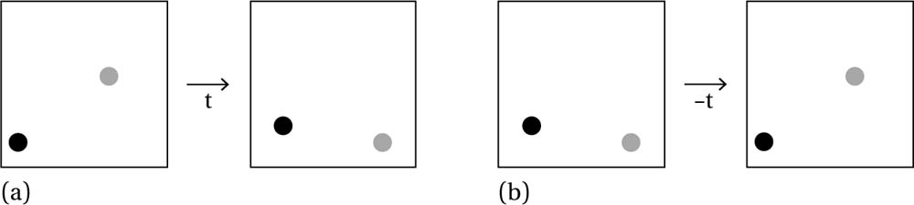
Fig. 6.3 Worldlines of two particles in relative motion where (b) is the time-reverse of (a).
The simplest way to explain this time symmetry is to invoke a movie of a bunch of atoms colliding like billiard balls. Watch such a movie for ten seconds, with the atoms going in their various directions. Then play the movie backwards. Both would be perfectly acceptable time evolutions for such a system (i.e. they are possible solutions of the equations of motion). For example, in figure 6.3 we see two movies with the same two particles. In the first movie (a), the dark particle moves up and to the right, just a small distance, while the light particle moves down and to the right, more quickly (covering more distance). In the second movie (b), the particles begin in the final position from movie (a) and end in the initial position of movie (a). In terms of laws, this amounts to inputting (a)’s final state as an ‘initial condition’ into the mechanical laws and generating (a)’s initial state as an output (this can be achieved by changing the signs of the particles’ velocities).
If we were to focus entirely on the particle worldlines for this ten second period, we would see that they were identical - see fig. 6.4. The form of Newton’s third law of motion, ![]() , makes this self-evident since the second time derivative doesn’t care whether we use t or −t - note that dependence on the second time derivative is not a necessary condition for time-reversal invariance; it just happens to be responsible in this Newtonian example. This means that if x(t) is a solution (corresponding to the trajectory shown in movie (a), then so is x(−t) (corresponding to the trajectory shown in movie (b), with the physical solution given by the equivalence class of time-symmetric solutions, as sketched in fig. 6.4.
, makes this self-evident since the second time derivative doesn’t care whether we use t or −t - note that dependence on the second time derivative is not a necessary condition for time-reversal invariance; it just happens to be responsible in this Newtonian example. This means that if x(t) is a solution (corresponding to the trajectory shown in movie (a), then so is x(−t) (corresponding to the trajectory shown in movie (b), with the physical solution given by the equivalence class of time-symmetric solutions, as sketched in fig. 6.4.

Fig. 6.4 Worldlines of the two particles from the previous movies, which you can think of as a photographs with a ten-second exposure time. Naturally, this picture would be the same for t and −t cases.
So the challenge for the theory is to find a way of getting time-asymmetric processes out of the time-symmetric laws, the former somehow emerging from the latter. Putting it in terms from above: how do we get time-asymmetric macromovies from time-symmetric micromovies? If it is possible (in terms of the microlaws) for all of the particles in a gas to undergo inverse motions (e.g. by flipping the signs of particle velocities), of a kind corresponding to the time-reverse of the gas in the box (or elevator!), then why do we not observe such things happening? From whence the arrow of time?
Ludwig Boltzmann attempted to resolve these problems after they were raised by Josef Loschmidt - the point is known as “Loschmidt’s Objection.” The crux of it is that given the time-symmetric nature of the laws governing the particles making up macroscopic systems, we ought not to see time asymmetric behavior. Entropy decreasing jumps, such as spontaneous coffee/milk unstirring should be observable. As philosopher Huw Price puts it: symmetry in, symmetry out. Conversely, to get an asymmetry out demands an asymmetry in the input. This input asymmetry, as discovered by barrister-turned-physicist Samuel Burbury, is the assumption of molecular chaos: pre-collision particles (i.e. their velocities and positions) are uncorrelated (probabilistically independent: random), but not so post-collision. In other words, the collisions of the particles are responsible for the observed entropy increase such that for any given distribution of states of the particles, it will inevitably evolve into an equilibrium state (the maximally random Maxwell state). Of course this leaves a problem that we will turn to in §6.7: if the system is already in a high entropy state, then it has nowhere to go. One needs some asymmetry in the dynamical evolution, but also an asymmetry in the boundary conditions: one needs lower entropy in the past so that the dynamical asymmetry can generate its effect.
6.3 The Laws of Thermodynamics
I hope you’re drinking a nice cup of tea while reading this book. When you pick up that cup (if you don’t have one, perhaps make yourself one), you are doing work of course - battling against the forces of gravity. The work converts kinetic to potential energy as you hold it up, which if (don’t try this bit) you should let go of the cup, will be converted into kinetic energy as the cup falls to the floor, shattering and spilling the lovely tea everywhere. Where does the energy go once it is lying in a mess on the floor? It went into thermal energy of the pieces and tea, and the floor and the air - of course, some of the energy already went toward heating up the air molecules in the cup’s path on the way down, subjecting it to air resistance. This is an example of the so-called first law of thermodynamics: total energy is conserved in a closed system (roughly, the room in which the cup was dropped immediately after it was dropped). The energy in this case was transformed between various forms: potential → kinetic → thermal - where the latter is, once analyzed, simply another form of kinetic energy (namely, that of the particles). Pre- and post-process (cup dropping) energy is a conserved (invariant) quantity.
There are certainly some interesting issues surrounding the first law, not least connected to the issue of ‘open’ versus ‘closed’ systems, which it involves. However, the real philosophical meat is to be found in the second law.
The second law can be seen in the same example: whereas initially the energy could do work - e.g. imagine a pulley system in which one end of the rope is attached to the cup and the other to a small mass (sitting on the floor perhaps) weighing less than the cup, so that dropping the cup from the table would see the mass rise - afterwards, when there is only thermal (random) energy, one cannot do useful work anymore, despite no loss of total energy in the whole system. Initially, there was a cooperation on the part of the molecules making up the cup and tea within it; a team effort of motion toward the floor. In other words: order. Afterwards, once it has come to rest, randomness prevails, with the molecules whizzing in all directions. This would be an equilibrium state - of course, equilibrium here does not mean some kind of zen-like ‘still point.’
The concept of entropy is at the root of the second law. Rudolf Clausius, building on Sadi Carnot’s work on the efficiency of steam engines, introduced this concept and with it the law to which it is associated. Clausius was interested in the movement of heat (thermodynamics), and noticed that it has a curious uni-directionality: objects initially at different temperatures when placed together so they are touching, will approach the same temperature. But this process of balancing has an endpoint at which there is no more flowing of heat across from the hot body (or gas) to the cold one: the heat gradient that existed earlier is no longer there. This never happens in reverse: hence, the second law - in this case, a matter of finding a balance so that the temperature is uniform (that is, at equilibrium). ‘Entropy’ was Clausius’ term for this tendency.
As with the first law, we need to include a statement about ‘closed’ versus ‘open’ systems, since clearly we can sometimes heat things up (the tea in your cup, for example) and cool things down (the milk for your tea from the refrigerator). Both require the input of energy, and the energy must exist in a low-entropy form (or lower than the system to which it is introduced) in order to perform work.
This takes us back to the first law, which, though it demands conservation of energy, does not forbid it from taking different forms. Some of these forms are more capable of doing work than others, and these are precisely those with the lowest entropy. Going back to the pre- and post-broken teacup, we can see that the pre-broken cup was in a lower entropy state than the post-broken cup since we could do some work with it (e.g. lift some object, as mentioned earlier, or use its more concentrated warmth to heat something).
These laws are of a similar kind in that they involve comparing quantities before and after some process has occurred. However, in the case of the first law, there is an invariance of a quantity before and after, in the case of the second law there is an inequality (always involving a quantity being larger than before). The quantity in the latter case is entropy S, to which we turn next. We also find that the second law, though it appears exact, was later understood to be probabilistic (i.e. true in the vast majority of situations). The concept of entropy is modified accordingly, and becomes a statistical concept (roughly having to do with the number of ways a state can be realized by its parts).
6.4 Coarse Graining and Configuration Counting
Our modern notion of entropy comes from Ludwig Boltzmann (superseding the more phenomenological version due to Clausius, relating entropy to energy and work). In a nutshell, Boltzmann’s idea is that entropy has to do with counting possible states for a system. However, we must split the types of possible state into two families, depending on whether they refer to the level of particles or the level of the systems made up of lots of particles. High entropy then simply means there are lots of ways for some state to occur (at the level of individual particles), and low entropy means that there are very few ways for some state to occur (at the level of individual particles).
The definition involves a mathematical procedure known as ‘coarse graining,’ which, as the name suggests, neglects certain fine but observationally irrelevant details of macroscopic properties. Starting with a system’s phase space, one divides it into cells, such that all of the phase points within a cell (henceforth: ‘microstates’) correspond to one and the same macroscopic state (henceforth: ‘macrostate’). In other words, the cells are equivalence classes where the relation of equivalence is ‘has the same macrostate as,’ which just means that one would not be able to distinguish between those microstates by observing the macrostate. An assumption of equiprobability is then made, such that each microstate is just as likely as any other. Crucially, this does not mean that each macrostate is equally as likely to be realized as any other: those macrostates that are associated with more microstates clearly have an advantage.
Let’s bring in a few technical details here, which aren’t so difficult - some of which we encountered in earlier chapters. Firstly, recall that the phase space (i.e. the state space) is understood to represent the space of possibilities for a system, here of n (indistinguishable) particles - indistinguishable, but still distinct and countable (giving the so-called Maxwell-Boltzmann distribution). Since it includes information on both the positions q and momenta p (for each particle) it will be a 6n dimensional space, which we call Γ. The idea of partitioning the space into cells is that while all points x = (q, p) represent physical possibilities, some points are to be seen as representing, many-to-one, the same possibility (in terms of macroscopically observable quantities): the physically measurable quantities one is interested in will be insensitive to differences amounting to swapping any such points. One can then think of the cells as themselves being the mathematical entities that correspond one-to-one with macrostates, so that each cell corresponds to a macroscopically distinguishable feature of the world. We can label each cell by coordinates wi, and let us also represent the volume of each cell by Wi (see fig. 6.5).
This small amount of apparatus allows us to now introduce Boltzmann’s famous equation for the entropy S of system in state x, where x ∈ w (that is, the state x of the system lies within the cell w). It simply tells us that the entropy is the natural logarithm of the volume of the phase cell in which it sits:
S = klog W(6.1)
It is then easy to see that the larger the volume W of the cell w that the system’s state x lies within, the more ways there are to ‘get’ that state; the higher the entropy will be; and (Boltzmann argued), the more likely it will be to occur.
Putting it back in terms of micro- and macrostates: macrostates realizable in more ways have a higher entropy and are more likely. For example, W tells us how often we can expect some temperature (of say 30° Celsius) to be realized. (Note that the number k is Boltzmann’s (conversion) constant used simply to get the two sides to agree in terms of units: k = 1.38 × 10⁻²³J(oules)K(elvin)−1. It can be viewed as a bridge, linking microscopic properties of individual particles (energies) with macroscopic parameters, such as temperature. The logarithm is used to get a grip on the huge numbers of microstates that some macrostates will be realizable by.) The largest cell will be that corresponding to the (thermal) equilibrium state, with the most microstates. This has the largest entropy. Hence, in much the same way as it is overwhelmingly likely to pick a red ball from an urn with 99 red balls and one black ball, so it is overwhelmingly likely to find the above system in a larger-volumed cell (assuming, as indicated above, that all of the microstates have an equal chance of being realized). The probability of some state is simply given by its volume (viz. the extension in phase space). The most probable state is then that realizable in 1, the most ways - this was called the Maxwell state by Boltzmann, since it conforms to a distribution discovered by James Clark Maxwell. This is the state that will found to occur most frequently and allows one to recover the (previously mechanically inexplicable) second law:
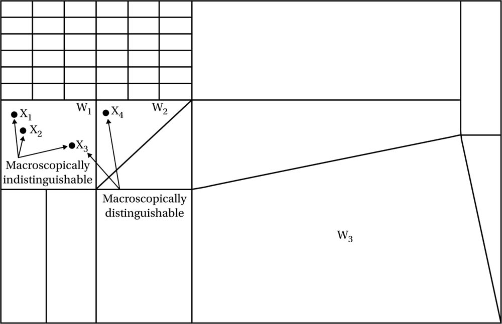
Fig. 6.5 An exaggerated example of a coarse graining of phase space ![]() into cells wi of volume Wi. The phase points (microstates) x1, x2, and x3 in cell w1 are indistinguishable (correspond to the same macrostate), while these points and x4 in cell w2 are distinguishable. Cell w3 has the largest volume (i.e. the greatest number of microstates capable of realizing it). It can be seen that W3 > W1 > W2. The geometry of phase space tends to make it overwhelmingly likely that the system will be in the cell w3 where it will spend most of its time.
into cells wi of volume Wi. The phase points (microstates) x1, x2, and x3 in cell w1 are indistinguishable (correspond to the same macrostate), while these points and x4 in cell w2 are distinguishable. Cell w3 has the largest volume (i.e. the greatest number of microstates capable of realizing it). It can be seen that W3 > W1 > W2. The geometry of phase space tends to make it overwhelmingly likely that the system will be in the cell w3 where it will spend most of its time.
![]() (6.2)
(6.2)
But it is, of course, a statistical explanation: it is probabilistically extremely likely to see the second law satisfied by the kinds of processes we are capable of observing because we are dealing with such large numbers of particles, which makes it vastly more likely that they don’t spend time in macrostates with less microstates.
Now, though this is rather elegant and easy to understand, there are all sorts of assumptions made, and there is an inescapable vagueness in the notion of “macroscopic indistinguishability.” One might easily be disturbed by the apparent looseness in doing the coarse graining: how is the carving up of the space carried out? How do we know that my carving will be the same as yours? Much depends on pragmatics: what level of precision is required? If you need to distinguish states more precisely than me, then you will use a finer ‘mesh’ size to cast into phase space, trawling for classes of indistinguishable states at that grain. Moreover, given that the entropy involves the logarithm of the cell volume, our distinct carvings would have to differ radically to get appreciable differences for S.
However, this understanding of entropy also has important consequences for some of the puzzles about asymmetry in time. The basic idea is that the number of ways to be in a ‘disordered’ (high entropy) state is greater than the number of ways to be in an ‘ordered’ (low-entropy) state (the volumes of the former will be greater than the latter), so we should expect an increase in randomness. Indeed, Boltzmann argues that a closed system driven by random collisions of particles should tend to maximum entropy (such as occurs when our initially localized fart from above spreads maximally throughout the elevator). This result, known as ‘the H-theorem,’ accounts for the derivation of temporally asymmetric behavior from temporally symmetric microscopic behavior - ‘H’ itself is a measure of deviation from maximal entropy, or the ‘Maxwell state’ (so that H is only found to get smaller over time). The probability for deviations away from the random Maxwell state will be smaller as the deviations become larger (by ever greater amounts). And, indeed, if one begins in a state that deviates significantly from maximal entropy, then it will have a large likelihood for approaching the higher entropy state. According to a common view, this is significant from the point of view of explaining the arrow of time: if the universe started off in a very improbable state (exceedingly far from maximum entropy), then it will have an exceedingly large likelihood of ‘making its way back’ to maximum entropy (via a sequence of higher-entropy states).
Let us now turn to the connection to such temporal matters.
6.5 Entropy, Time, and Statistics
The second law is probably the most well-known (and seemingly solid) law of nature. It says, quite simply, that entropy (for closed systems) never decreases - of course, one could ‘open up’ such a system and pump energy in, thus lowering the entropy (as happens when we clear the messy dishes and place them in the dish rack, for example). Much of the fun stuff in the philosophy of thermodynamics comes out of Ludwig Boltzmann’s statistical (microscopic) explanations of thermodynamical behavior. Prior to the microscopic understanding he provided, the laws were understood in terms of the ability of systems to do work (such as powering a piston) or not. Entropy was then understood in terms of degrees of irreversibility.
Take my daughter Gaia’s room, for example (see fig. 6.6). It is seemingly always in a state of near-maximal disorder. To impose order requires me to input energy (cleaning it: in which case it isn’t a closed system): hence, it becomes an ‘open system’ and does not ‘naturally’ tend to an orderly state. There are very few ways for it to be clean and orderly (with books organized alphabetically, and so on), and very (very) many ways for it to be disorganized. In terms of ‘energy cost,’ it is far cheaper to bundle books and clothes haphazardly than to have them arranged neatly - something Gaia knows all too well… Hence, there is a nice intuitive way of understanding entropy in terms of possibilities: it provides a measure of the number of possibilities for realizing some system state or configuration. Messy rooms can be realized in more ways than tidy rooms. It would not be a good strategy to randomly throw objects into positions: the number of tries it would take to ‘fluke’ the tidy configuration would be of the order of very many googolplexes (which, in temporal terms would be very many times the age of the universe)!

Fig. 6.6 A messy bedroom: by far the likelier configuration. Relating this back to the coarse graining diagram, we could expect this to be represented by w3, or one of the larger cells. Tidying the room ‘pushes it’ into one of the smaller cells. The second law then results in a motion toward the largest cell once again, so long as external energies (e.g. cleaning) are not put in.
Aside: The ‘intelligent design’ brigade like to abuse this kind of reasoning to argue that the magnitude of order in the universe (particularly in the biosphere) can’t be accidental since it’s too improbable - like fluking the tidy bedroom configuration by randomly throwing objects about. So, they say, it must have been designed this way by a superior intelligence.
The problem (one of many…) with this argument is that the steps leading to ‘the accident’ would have to be uncorrelated (random) for this to work. But they are not random: evolution by natural selection is a law-based cumulative process involving vast timescales.
To repeat: Boltzmann’s neat formula expresses this relationship between the degree of disorder (entropy, S) and the number of ways that the system can be organized (or disorganized).1
This brings us back neatly to what is probably the most studied (by philosophers) aspect of thermodynamics: the appearance of an asymmetry of time, often called time’s arrow. Our memories are of the past: the future is out of bounds. Yet, it appears that we have some degree of influence over the future, but not the past.
A common explanation for this asymmetry ties it to another asymmetry: that embodied in the second law. Since there seems to be an in-built irreversibility to the universe (entropy only increases and is irreversible for all practical purposes, with an unflinching march of order into disorder), the explanation for time asymmetry can ‘piggy back’ on this ‘master arrow.’
Firstly, let’s recall what is meant by “temporal asymmetry.” What it indicates is that the laws (or phenomena described by some laws) are not time-reversal invariant. That is, the laws distinguish between a video of some process played forwards and backwards.
Think of the universe as rather like a grand version of my daughter’s bedroom. We ought to expect, given Boltzmann’s reasoning, that we should find it in a state of disorder (one of the larger cells). But, puzzlingly, we don’t. We see an awful lot of order. Hence, from this perspective, our universe is very unlikely. Of course, we always knew there was something strange about it, but we can now quantify how odd it is.
Indeed, given our ordered state, we ought certainly to expect that the entropy goes up in the past, since there are more ways to be in high entropy states. This was the case according to Boltzmann’s theory (which, according to him, ‘boldly transcended experience’), who believed that the order we find is indeed highly improbable, but is bound to happen given unlimited time.
This explanation of time’s arrow (by attaching it to the direction of increasing entropy) suggests that entropy-increase should be more probable both to the future and the past: there should still be a time-symmetry. The problem is, for some ordered state, it is more likely to have come from a less well-ordered state simply because those less ordered states far outweigh the ordered ones. Hence, Loschmidt’s reversibility objection strikes again. We turn to Boltzmann’s ingenious solution (invoking cosmology and the Anthropic principle) in a moment, but first let’s consider another problem that faces the statistical account.
6.6 Maxwell’s Demon
Recall that the second law states that entropy (in closed systems) is (for all practical purposes) unidirectional. In the second half of the nineteenth century the law was well known, and had already been tied to dire predictions about the fate of humanity: if useful mechanical energy steadily dissipates, then there’ll be no power to run the world (and nature), with all energy eventually becoming thermal, random energy - you can’t power anything with the ash from a fire. But recall also that the laws governing the particles’ behavior are not necessarily unidirectional. Since the entropy changes are a result of the motion of the particles (i.e. it supervenes on the particles’ properties), there seems to be no reason why the second law should hold (this is Loschmidt’s objection again). By focusing in on the individual particle level, James Clerk Maxwell proposed a way of beating the second law (and the unhappy fate for humanity). It’s a very simple setup, and really it doesn’t demonstrate the falsity of the second law as such, but rather reveals its statistical nature - mentioned already, of course, but which found its earliest well-posed formulation in Maxwell’s argument.
One imagines a box of gas, at some given uniform temperature, with the individual gas molecules buzzing around at different speeds (the average giving the temperature of the whole). Then one imagines placing a wall down the middle, dividing the box into two smaller boxes, and with a smaller hole in the partition that can be opened and closed at high speed (see fig. 6.7). We suppose that the two sides have the same number of molecules, and that they are at the same constant temperature. The two sides are at equilibrium relative to one another and in themselves. Though they are at equilibrium (so their mean temperatures are identical), the particles within will differ in speed at an individual level: some will be faster than others.
Next comes the demon, clearly based around Laplace’s (in that it has access to the positions and momenta of all of the individual molecules in a system). It is really just a very high-speed sorting device that can keep track of the various particles whizzing around in a gas. The demon is able to allow fast moving particles through the hole into the left-hand side, say (quickly opening it as they approach), and keep the slow moving particles in the right (by quickly closing the hole). This sorts the two sides of the box into hotter and cooler gases, thus generating a temperature difference capable of doing work (such as driving a piston), yet apparently without doing much work to create it. The idea is that the demon apparently violates no laws of molecular physics with its actions, and yet has the effect of decreasing the entropy in the box. If this is a possible scenario, then it amounts to a perpetual motion device, since one is generating the energy version of a free lunch!
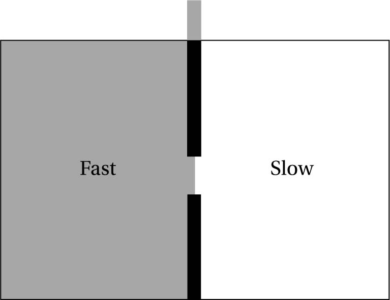
Fig. 6.7 Simple representation of Maxwell’s Demon: by judiciously opening and shutting a door, a demon would be able to sort the particles so that hotter and colder regions are formed from a system initially in or close to equilibrium, in violation of the second law.
We all know there is no such thing as a free lunch, so to preserve the second law (statistical or not), we need to explain the apparent violation away. One way in which it could be preserved is if the missing entropy showed up somewhere else, such as the opening and closing of the shutter or the demon’s own actions. Rolf Landauer famously argued that provided the demon recorded the measurements (with perfect precision) then the process he carried out would be perfectly reversible and therefore not entropy-increasing: if a record of some process exists, then the process is reversible; if not, then it is irreversible, and such irreversibility is the hallmark of entropy. The problem is, it would require a vast amount of memory resources to keep track of all those processes. In order to keep track, it would have to wipe its memory now and again. But this would make the process irreversible (leaving no record with which it could restore the earlier state), thus safeguarding the second law. Hence, Maxwell’s demon needs to be absent-minded for the example to perform its function. However, wiping a memory creates entropy since the states held in the ‘memory register’ are shrunk down to one (0, say).
Other versions of Maxwell’s demon come in the form of gravity, and more specifically via aspects of black holes. Black holes are defined by just three numbers: their mass, charge, and angular momentum. This enables a certain amount of ‘forgetful’ behavior that appears to offer a way to violate the second law. Simply throw a highly entropic object (such as the broken teacup) into the black hole and voila: the breakage never happened and the entropy is erased from our universe! However, this situation is avoided (and the second law saved) in virtue of a correspondence between entropy as usually conceived and the area of a black hole’s event horizon: the latter only ever grows, by analogy with the former. So when we toss in our broken teacup the horizon increases by a tiny amount, increasing the overall entropy in the universe - analogous versions of all of the laws of thermodynamics can be found.
Zermelo had objected to Boltzmann’s statistical account of heat by invoking Poincaré’s ‘recurrence theorem.’ He points out that given infinite time, there will be a perpetual cycling through all possible states, so that motion is periodic rather than settling into some fixed Maxwellian distribution. In other words, the distribution of states should be flat (with no preferred equilibrium value) since they will all be realized infinitely often. Again, at the root of the confusion appears to have been a breakdown of intuitions where very large numbers are concerned. When one compares the states that deviate from maximum entropy states with the maximum entropy state, one finds that there are vastly more ways of realizing the latter than the former. The problem Zermelo had is in understanding the fact that though the Maxwellian macrostates appear to be few, they preside over the greatest volume of microstates. By pointing to the statistical nature of the laws, Boltzmann brings statistical mechanics within the recurrence theorems. It is quite simply that any such recurrences are so improbable as to be rendered unobservable within any reasonable amount of time (what Boltzmann himself called a “comfortingly large” time). That is, the magnitude of the improbabilities means that they are ignorable for all practical purposes.
Of course, philosophers are not known for their adherence to practicalities, so we might still be rightly concerned by the conceptual implications of Boltzmann’s view, for it indicates that we are simply around because of an improbable fluctuation in a vast bath of thermal energy that has existed for a very long time. Besides, Zermelo responded by pointing to a glaring hole (noted by Boltzmann himself) that we have no physical explanation for why the initial state (our ordered universe for example) has such a low entropy. Boltzmann thought this was akin to explaining why the laws of nature are as they are, and as such transcended physical explanation: one would be explaining the grounds of explanation.
6.7 The Past Hypothesis
Entropy is, to a rough approximation, disorder. It increases with time. That is a puzzle: why should it do that? But entropy was lower in the past than it is now. That is also a puzzle: why exactly is that? This is a quite different problem then. We have discussed the issue of why entropy increases to the future. But now: why does it decrease into the past? If there are more ways for our universe to be disordered rather than highly ordered, then why is it more highly ordered now? Why isn’t the entropy much higher in the past as we move away from our present low-entropy condition (a question Boltzmann asked himself, prompted by Loschmidt’s complaints mentioned above)? This points to a serious conflict between our knowledge of the world and our experience of that world: our memory records (of, e.g. cups of tea that were not shattered on the floor) are more likely to be false than true, since the events they seem to concern are improbable (thanks to their lower entropy than the present condition).
Boltzmann indeed surmised that followed far enough into a distant past, we would find maximal entropy there too (molecular chaos), just as in the future. The asymmetry smears out over long enough temporal journeys. This is truly a mind-bending proposition, every bit as radical as the idea that the Earth is not at a distinguished point of the universe. It might seem that if we know why it goes up in the future (using Boltzmann’s idea that the increase would be perfectly natural if the past contained a local fluctuation of very low entropy) then we have explained the arrow. But we are left with a puzzle about the past in this case.
One explanation, that we have already met in connection with time’s arrow, is to simply postulate a low-entropy past (the ‘past hypothesis’: a label due to David Albert). This is usually attributed to special conditions of the Big Bang in our universe’s past. Hence, the idea is that if our universe began in an immensely low-entropy condition, then it can’t help but to increase in entropy, such as we find (as mentioned above).
To attempt to explain the increase of entropy by postulating a low-entropy past simply introduces another problem (or, in some ways, recapitulates the same problem): how do we then explain the low-entropy past? It is not enough to point to the Big Bang and utilize the apparent low entropy found there, since that very order is what is in need of explanation. Passing the buck onto something so incredibly improbable as the Big Bang leaves us no better off. However, the past hypothesis does have the considerable virtue of defusing the Loschmidt reversibility objection: our time asymmetry (linked to the entropy-asymmetry) rests on the existence of asymmetric boundary conditions. The unlikely configuration at the absolute zero of time as we know it (the Big Bang event) means that whatever patch of order we find, we know that preceding it will be a patch of lower entropy, tracing all the way back to the initial temporal boundary that the Big Bang provides (and at which we impose our boundary condition).
But even supposing we could resolve this issue, how plausible an account of time’s arrow is it anyway? How plausible is it that all of those many irreversible features - including the asymmetries of our memory records, the non-unmixing of our tea, our unfortunate ageing - are due to something that happened around fourteen billion years ago?!
One way to think about this is to imagine what the world would look like if we had reached a state of maximal entropy, an equilibrium state in which there is one temperature for all. Would there be a direction of time in such a world? It’s hard to see how asymmetric processes could be taking place. To use the standard metaphor of running the video of such a world backwards, we would find no distinction, and hence there would be no physically observable arrow of time. Though we could still speak of a second law in operation in such a universe, there would be nothing for it to ‘act on’ as it were. There would therefore be no temperature gradient, no entropy gradient. So we can see how having an entropy gradient is necessary in some sense to allow the sorts of time-invariant changes we experience, and if the gradient ‘flows’ to a state of maximum entropy, then we can see how the story is supposed to work. But a necessary condition is not quite the same thing as an explanation.
In one sense, it is good to ground universal behavior in a common origin. However, again, the way this is done in the present case simply pushes the mystery of time’s arrow one step back. We immediately want to ask: why those initial conditions? Unfortunately, our present physical theories don’t enable us to provide an answer - though plenty are trying!
There are two options: explain the present improbability, or don’t. Boltzmann was in the latter camp, not thinking it plausible to deduce our improbable past and present from fundamentals. For Boltzmann the universe at a large scale is in thermal equilibrium (as the most probable of all states), and our existence is due to a local deviation (a quirk of probability) - see fig. 6.8.
To wax lyrical for a moment: we are born of random fluctuations, and will return to random fluctuations. Hence, he denied any fundamental status to the arrow of time, viewing it as a purely local phenomenon, much as the convention of ‘up’ and ‘down’ on the Earth is local (see fig. 6.9). The arrow of time stems from an Anthropic coincidence, that there happen to be sentient creatures (us) supported by the local fluctuation. Given our circumstances, of finding ourselves in an ordered world (how could it be otherwise if we are to exist?), we will see an arrow of time in which the improbable order moves to disorder. And the crucial point is this applies to both directions of time if one looks far enough back (i.e. to before the low-entropy blip). Boltzmann predicted, from his analysis, the existence of a kind of multiverse picture, in which scattered about the universe, which, remember, is in thermal equilibrium (essentially dead, with no elbow room to increase in entropy), there are worlds like ours (fluctuations about equilibrium), which depart from equilibrium for short times compared to the timescale of the entire universe (see fig. 6.8). Just as in modern multiverse theories one needs an enormous amount of worlds to explain the existence of our apparently fine-tuned universe, so for Boltzmann one needed an immensely vast universe in thermal equilibrium to explain our world - see §8.7 for more on Anthropic reasoning. Were we not seeing an arrow of time, the entropy would be too high for an arrow to emerge (not enough gradient), and so we wouldn’t be here to consider it. In other words: wherever there be observers, there be an arrow of time. It couldn’t be otherwise. Moreover, the local conditions would dictate which direction would be considered ‘future’ and which ‘past’ (see fig. 6.10).
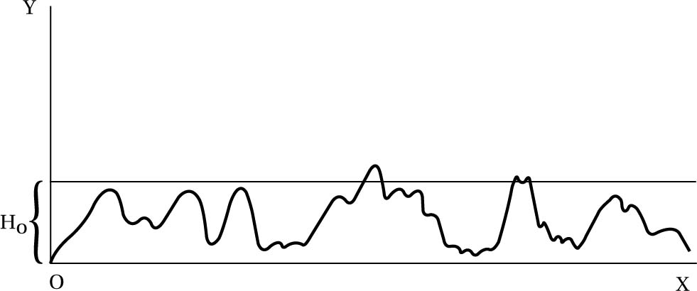
Fig. 6.8 Boltzmann’s diagram showing the local deviations from thermal equilibrium. Reproduced in S. Brush, ed. The Kind of Motion We Call Heat (North Holland, 1986: p. 418). Here H is a quantity that Boltzmann himself used, inversely related to entropy: when it is low, entropy is high and vice versa. The curve represents the history of the universe, where the highest peaks (or “summits”) correspond to phases potentially containing life (such as our own world): the larger the peaks, the more improbable the state. (Here γ is the ‘extension’ of the state giving its probability of occurrence and x is the temporal direction.)
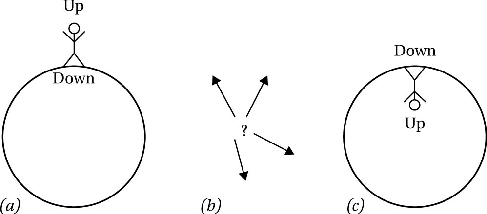
Fig. 6.9 ‘Up’ and ‘down’ orientations are locally defined relative to reference frames. In (a) and (c) a person’s conventions for orientation will be distinct depending on whether they live on the surface of a sphere (such as the Earth) or in the interior of a sphere (such as aboard a rotating spaceship). With no such reference systems to fix a convenient orientation convention (as in (b)), ‘up’ and ‘down’ are meaningless.
Other attempts at an explanation focus on aspects of early universe physics in an attempt to fill in the details of the ‘special initial conditions.’ One famous example of this, due to Roger Penrose, invokes the ‘Weyl curvature hypothesis’ - where the Weyl curvature tensor tracks aspects of the curvature of spacetime that would be found in space emptied of all but gravitational field (matter is ignored here since it is believed to be at maximal equilibrium in the earliest phases). Penrose’s hypothesis is that this entity vanishes near the Big Bang singularity and implies a low entropy there. But this won’t do as an explanation of the past hypothesis (the special initial state); instead it reformulates the past hypothesis in terms of the Weyl tensor. Why do we have the vanishing Weyl tensor is simply a way of re-expressing the original puzzle. Indeed, Penrose passes the buck to a future theory of quantum gravity that would be able to deal with situations in which gravitational fields are incredibly large, and quantum effects must come into play.
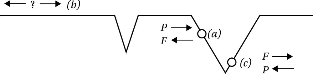
Fig. 6.10 By analogy with the ‘up’ versus ‘down’ scenario, here we see three possibilities with respect to time’s arrow: in (a) the past runs toward the right (and the future to the left), since that represents a decrease in entropy (a larger deviation from the thermal equilibrium); in (c) the past runs toward the left (and the future to the right), since that represents a decrease in entropy relative to its location; in (b) there is no entropy gradient to determine an arrow of time.
We saw earlier that Zermelo was in the former camp (explain the improbable state) - or at least, he viewed the bruteness of the improbability as a problem for the statistical-mechanical approach. Boltzmann thought this was unprovable and had to be assumed.
In terms of explanation of the low entropy, one might extract an Anthropic explanation from Boltzmann’s own arguments as above. After all, he believed in what is essentially a vast ensemble of worlds, and what kind of world would we find ourselves in but one with a low entropy past? Of course, as an explanation it is weak, since we aren’t deriving our world from the scheme, only showing how they are compatible (which was all Boltzmann was concerned with). When we push Boltzmann’s idea, however, we find it faces a curious problem (perhaps a reductio ad absurdum), which we turn to next. The problem, simply put, is that if it’s consistency with observable results that we’re after, then it can be achieved on a tighter entropy-budget than generating an entire universe that has persisted for billions of years: what a waste of effort! If one could get the same effect (a universe, that appears to have existed for billions of years, with star formation, the evolution of life, etc.) from a much smaller fluctuation - say a single Cartesian-style disembodied brain configured with the correct memories, believing it has had the ‘correct’ experiences, and so on - then, given the inverse relationship between the magnitude of the fluctuation away from thermal equilibrium and the probability of such a fluctuation occurring, this brain scenario would be vastly more likely. This is, of course (I hope!), absurd. If we are bothered by the problem of other minds (so that we cannot countenance solipsistic single-mind views of the universe), then there are still many more likely scenarios than having the universe actually be as old as it seems (which is a persistent fluctuation, and so less likely than a shorter-lived one): the theory that the universe came into existence five minutes ago (fully formed) is far more likely in terms of the likelihood of such a fluctuation relative to an extended one trailing billions of years into the past.
6.8 Typing Monkeys and Boltzmann Brains
Fans of The Simpsons might recall the episode ‘Last Exit to Springfield,’ in which a kidnapped Homer is shown a room in Burns’ mansion in which a thousand monkeys are typing away, with one typing the almost correct “It was the best of times, it was blurst of times,” from Charles Dickens’ A Tale of Two Cities. The so-called ‘monkey theorem’ tells us that given enough patience (and time for that patience to manifest itself), and some monkeys randomly thwacking keys on a computer, we can expect to see generated the complete plays of William Shakespeare. One would, in fact, require a lot of time: far more than the present estimates for the age of the universe (about fourteen billion years). Amusingly, a computer programmer, Jesse Anderson, attempted to approximate this by simulating millions of monkeys (‘virtual monkeys’), which churn out random ASCII characters between A to Z, which are then fed to a filter to test for fit with actual lines of Shakespeare (as found on Project Gutenberg) - the results are as expected: one can randomly generate such apparently meaningful segments given time enough and monkeys or monkeys enough and time (i.e. processing power capable of generating the appropriate output strings). Of course, each string is as random as the other (by construction), but we see order in certain strings. To get a handle for how approximate such a simulation would be, just consider that for a work with 500,000 characters (a reasonably sized novel), the probability of getting the novel churned out in this random way would be 2.6 × 10−500000 (3.7 × 10−500000 if we add numbers 0 to 9 and blank spaces). By the same token, one can see that if time were no obstacle, it would happen sooner or later - hence, this is often labeled the ‘infinite monkey theorem’: one monkey with infinite time, or infinitely many monkeys with finite time, either will do the job.
We can play a similar game (known as Boltzmann’s brains) with atoms, time, and space, only this time constructing (now via fluctuations from the vacuum) any physical structure we could care to name, including ourselves and the entire observable universe. Indeed, given a universe with infinite time, you will be ‘reincarnated’ infinitely often: eternal recurrence! There are vastly more possible configurations than constrained by the choice of ASCII characters in this case, so the probabilities will be vastly smaller. But the point remains, given unlimited time, it would happen - the ‘principle of plenitude’ (that anything that can happen will happen) likes infinite time. (Interestingly, one can find a strikingly similar scenario painted in Friedrich Nietzsche’s combinatorial notion of eternal recurrence. Simply expressed, he points out that given some definite constant energy distributed over a finite number of particles, in infinite time every combination must already have happened, and infinitely many times, repeating in cycles as each initial state recurs. In Nietzsche’s mind this was supposed to be a victory against the materialistic physics that pointed to a winding down of the universe, in a final equilibrium state known as the ‘heat death.’ Yet what such recurrence objections reveal is that the second law does not apply universally, and that Boltzmann’s statistical, yet still mechanical, viewpoint is to be preferred.)
The implications here are similar to the classic ‘brain in a vat’ scenarios that epistemologists like to chew on. From the perspective of us, ‘inside our own skulls’ as it were, we can’t tell whether we have genuinely lived the lives we appear to have lived, having the various experiences that formed the memories we appear to have, caused by a universe that appears to be very old, and so on. We might be a disembodied brain in a laboratory undergoing stimulation and reconfiguration to generate such appearances. Our memories would not be records of real events; rather, they would be implants. As David Albert emphasizes, looking in history books for evidence is no good: they too are more likely to have fluctuated into existence without any causal link to the events (e.g. the rise and fall of the Roman Empire) they appear to describe - this is analogous to Dr Johnson kicking a rock to refute George Berkeley’s brand of skepticism about the external world.
Likewise, in the case of Boltzmann’s brains. In a universe that persists for long enough, there is a tiny but non-vanishing probability that a brain with all of your thoughts and memories, thinking it has lived a life having read books about physics and so on, will spontaneously generate. Given that the energy cost of generating such a region of order (the disembodied brain) is considerably smaller than generating an entire universe whose development over fourteen billion years led to it, it is more likely that we are such a Boltzmann brain than not! Boltzmann brains ought to be more typical than the long-haul brains we think we have. To put it another way: If you happened to be a god looking to create sentient beings, you would save a lot by just bypassing galactic and biological evolution, and having them pop into existence fully formed.
We have seen that Boltzmann’s explanation for the thermodynamical arrow of time (entropic increase) says that regions of time asymmetry are unusual: the usual state is one of molecular chaos. Hence, we are in a special state: time-symmetry is the norm. From this thermal bath, all manner of odd fluctuations can arise, with the size of their deviations from equilibrium linked to their likelihood of occurrence. Sean Carroll puts the point rather nicely:
[A] universe with a cosmological constant is like a box of gas (the size of the horizon) which lasts forever with a fixed temperature. Which means there are random fluctuations. If we wait long enough, some region of the universe will fluctuate into absolutely any configuration of matter compatible with the local laws of physics. Atoms, viruses, people, dragons, what have you. And, let’s admit it, the very idea of orderly configurations of matter spontaneously fluctuating out of chaos sounds a bit loopy, as critics have noted. But everything I’ve just said is based on physics we think we understand: quantum field theory, general relativity, and the cosmological constant. This is the real world, baby. (“The Higgs Boson vs. Boltzmann Brains”: http://www.preposterousuniverse.com/blog/2013/08/22/the-higgs-boson-vs-boltzmann-brains/)
If this is the implication of our best physics (as it seems to be), then I submit that it needs the urgent attention of philosophers (in addition to physicists)!
6.9 Why Don’t We Know about the Future?
This might sound like a silly question (the future hasn’t yet happened, stupid), but it clearly has to do with the arrow of time and, as we have seen, statistical mechanics and entropy are bound up with that. Perhaps, then, one can explain the ‘epistemic arrow of time’ (involving the past-future asymmetry of knowledge) by making use of some of these concepts? Since entropy increases from past to future, we need to make sense of how it can be that our present observations tell us more about the past than the future.
The classic example involves the notion of a memory trace. A trace is a low-entropy state. A memory record, for example, must be sufficiently distinctive to ‘make a mark’ on the host. Something that wasn’t there previously. One can think of this process (and the link to an experience of a flow of time: a subjective feeling of a sequence of events seemingly coming into being) in terms of the difference between randomness and order. A uniform, random experience or event (say of a perfectly flat featureless sandy beach) will not be distinguishable in itself (assuming all other conditions are kept fixed) from a snapshot of the same beach at a later time. However, if a wind stirs up a sand dune (especially if that dune takes on the appearance of some object or person, say) then it leaves a mark. It is a departure from randomness.
This (marks, traces, etc.) is really all we have to go on evidentially speaking, and so we make inferences about the past (retrodictions) just as much as the future (predictions). But we seem to have a stronger basis for past inferences: though I might be mistaken about the exact way in which some past event occurred (inferring from a memory or some other trace), I know that something happened; yet with the future we don’t seem to have such certainty - I might think ‘next Monday there’s a research seminar,’ yet some calamity could cause the speaker to cancel so that it doesn’t occur. So how does a notion of trace help here? Hans Reichenbach’s case of a footprint found on a sandy shore is a good example of a kind of trace. One can also readily see the link to entropic considerations. The footprint (trace) provides present evidence about what happened in the past. The idea is that the footprint ‘does not belong there,’ entropically speaking, relative to its surroundings, enabling one to infer that there was some kind of intervention (an outside influence) leading to its existence. In other words, the sandy shore is not a closed system, and an entropy-reducing process caused the local reduction in entropy characterizing the footprint in the sand. The shore’s entropy was lowered by something external: it can’t have been a closed system.
But just how relevant is entropy to such retrodictions from traces? John Earman argues that it is not at all relevant: one can just as well make past inferences on the basis of very high entropy. Low entropy is not necessary for traces, and one can imagine such things as catastrophes wreaking havoc on some orderly town, increasing the entropy there. Yet one could still make an inference, from the damage, that there was an intervention ‘from outside.’ Given the nature of the damage caused, one can even describe features of the causal influence (e.g. using the Saffir-Simpson wind scale and other such instruments). However, as Barrett and Sober point out, though the low-to-high transition of entropy is not at work, one should not rule out the importance of entropy in inference. One can say that, given the system (town, beach, etc.), there are certain expected entropies that if disturbed (in either direction) point to outside influences. But in such cases, background knowledge of the system (providing history and standard behaviors) is needed. Hence, the crucial aspect is that there is some departure from expected properties (such as entropy).
Note also that the marks seemingly provide evidence for our inferences about the past only if we accept the past hypothesis. It is the past hypothesis that provides us with the explanatory edge that we seem to have with the past over the future. Otherwise, we might infer that the fluctuation from molecular chaos story was the correct one (since it would be the most statistically likely). Some inferences about the past and future are balanced: those that come from the information about the current state combined with the laws, which allow us to propagate states in both directions. But we can do more into the past. Suppose, for example, that your mother walks in and sees the broken cup on the floor. She doesn’t assume it’s a random fluctuation, but that it was the result of an ordered causal sequence of progressively lower entropy states - unless she’s a physicist, she’s unlikely to think of it this way, but her thought-processes will be along just such lines all the same: ‘the cup was together in one piece, and contained hot tea, which involved it being contained within a kettle …’. (You might compare this additional way of reasoning with Laplace’s demon armed only with the laws and the initial state of all the matter in a system.)
Bizarrely then, the asymmetry of knowledge (and the function of memory) depends on the conditions many billions of years ago. If we didn’t utilize it (however implicitly) our reasoning about the past would be no better than about the future. Our reasoning about the future is uncertain about many things, but we know that molecular chaos will be the likely event of most present (well-ordered) conditions. The past hypothesis means that the same is not true of the past (and so the conditions that led up to the well-ordered present event). You might, as mentioned earlier, find the linking of memories (which are also clouded with all sorts of emotions) with the low-entropy past as too flimsy to really provide an adequate explanation. Still, it would then remain as a challenge to explain how memories give us information about the past.
To finish up this fascinating issue, I leave the reader to ponder what other areas of our inferential machinery are dependent on the past hypothesis.
6.10 Further Readings
Some excellent recent textbooks on the philosophy of statistical mechanics have emerged recently. Also, thanks to the links to such issues as arrows of time and knowledge there are also some fun, popular books.
Fun
· David Albert (2001) Time and Chance. Harvard University Press.
- Short and sweet! Essential reading for any philosopher of physics, and anyone wishing to understand the deeper implications of statistical mechanics.
· Sean Carroll (2010) From Eternity to Here: The Quest for the Ultimate Theory of Time. Dutton.
- Popular, and with sparkling examples, but the issues are presented with real depth of understanding.
Serious
· Huw Price (1997) Time’s Arrow and Archimedes’ Point: New Directions for the Physics of Time. Oxford University Press.
- Comprehensive treatment of time asymmetries covering some very difficult terrain in an easy to understand way.
· ✵ Lawrence Sklar (1995) Physics and Chance: Philosophical Issues in the Foundations of Statistical Mechanics. Cambridge University Press.
- Solid text covering virtually all the central topics in philosophy of statistical mechanics.
Connoisseurs
· Meir Hemmo and Orly Shenker (2012) The Road to Maxwell’s Demon: Conceptual Foundations of Statistical Mechanics. Cambridge University Press
- The focus is on issues of time asymmetry, but this book covers a very wide range of issues in the foundations of statistical mechanics in great depth and in an exceptionally clear way.
· Gerhard Ernst and Andreas Hüttemann, eds. (2010) Time, Chance, and Reduction: Philosophical Aspects of Statistical Mechanics. Cambridge University Press.
- State of the art treatment of time’s arrow, the meaning of probabilities, and reduction.
Notes
1 Though the association of entropy with disorder is problematic it provides a useful mental foothold from which one can view the more precise combinatorial landscape. Physicist Arieh Ben-Naim has gone to great lengths to correct various misunderstandings of entropy (including the disorder interpretation!). See his book Entropy and the Second Law: Interpretation and Misss-Interpretations (World Scientific, 2012) for a very useful treatment. For a more elementary exposition, see his Discover Entropy and the Second Law of Thermodynamics: A Playful Way of Discovering a Law of Nature (World Scientific, 2010).