The Philosophy of Physics (2016)

2
General Concepts of Physics

This chapter introduces, very briefly, several core concepts of physics from a bird’s-eye view, rather than up close in the context of specific theories (something we do in later chapters, for classical and quantum, statistical and non-statistical, and relativistic and non-relativistic physics). Here we find out about states (a full specification of a system’s properties, or values of all variables, at some instant), observables (those variables in a theory that can be measured and given a physical interpretation), and dynamics (the rules governing the behavior of a system, e.g. under the action of forces): the three core features that go into the construction of a physical theory and that form the raw materials for our interpretations. One finds these same basic concepts replicated across the theoretical frameworks above, where their specific realizations will differ according to the nature of the systems the theory is supposed to describe. These concepts are, then, at the root of the mathematical representations that we wish to make physical sense of. In particular, differences (of interpretation) can be seen to emerge within a theory about what kind of stuff the states and observables refer to. The dynamics enters this same interpretative debate in a variety of ways, especially in virtue of its link to symmetries - the next chapter puts these three basic concepts (states, observables, dynamics) to work in unpacking the concept of symmetry that will figure heavily in the remainder of the book.

2.1 The ‘Three Pillars’

Philosophers of physics often like to speak of the ‘pillars of modern physics,’ by which they have in mind the theories of relativity, quantum mechanics, and statistical physics. What they mean is that these three together provide frameworks for the rest of physics - whether they are directly employed or not, they are seen to underlie all other phenomena (see fig. 2.1). However, one shouldn’t take the ‘pillars’ metaphor too literally: they do not stand in isolation like architectural pillars, linked only by what they support or rest upon. Rather, as we will see, they overlap considerably. Perhaps a better metaphor is to think of them as distinct strands of fabric woven together to make up a single sweater (a very nice one, not like your granny might knit). The three pillars are all examples of spacetime theories: they include spacetime (or space and time) as one of the fundamental elements of reality. Spacetime (or space and time) is part of most representations employed in physics: if they are supposed to model the world, then they should contain space and time because this is how the world seems to be configured, at least at some level of approximation - some theories of ‘quantum gravity’ suggest spacetime is not a fundamental feature of reality, so that spacetime ‘emerges’ from some deeper non-spatiotemporal theory: we briefly discuss quantum gravity in §§8.4 and 8.5.

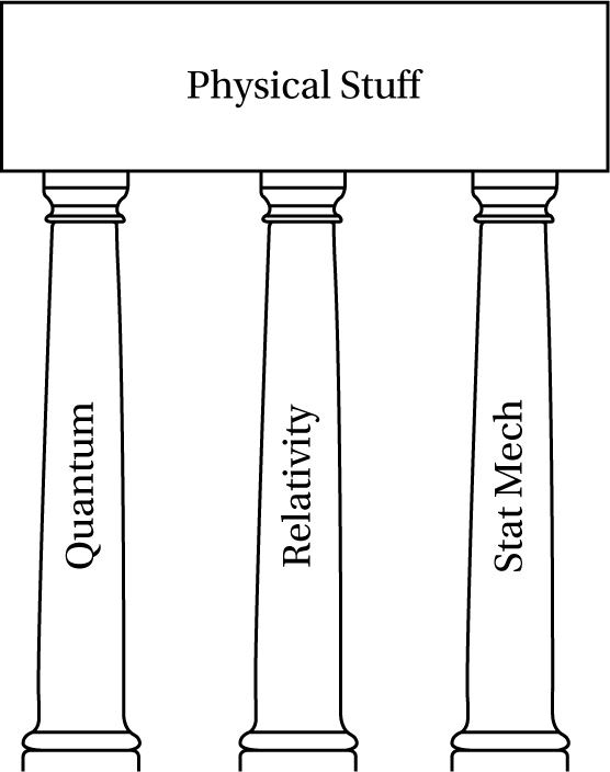
Fig. 2.1 The three pillars of modern physics: all phenomena of nature are viewed as reducible to three basic frameworks: statistical physics (often called ‘stat mech’), the theories of relativity (special and general), and quantum theory - a common, though rather inaccurate picture of modern physics.

Spacetime theories tend to match up with respect to their basic (deepest) structure: a set of points taken to represent the basic events of reality (or locations where events, such as colliding point particles, can take place) - however, some have argued that independently of further structure such ‘bare’ points can’t represent real physical stuff. Distinct theories then diverge according to what further structure is applied to this foundation, depending on what they wish the theory to represent. Onto this set of points we can lay ‘charts’ or coordinates, labeling them and allowing us to speak of the points’ relationships to one another - this set of points has the structure of a ‘manifold,’ namely something that ‘looks locally’ (i.e. at short distances) like ordinary flat space, but can vary in all sorts of ways globally (think of a newspaper laid flat versus rolled up: the way they differ is said to be a ‘global’ difference, but viewed up close enough there is no way to see such differences). We can map these points or regions of a manifold to itself (via transformations) to represent all sorts of possible changes (spatial movements, rotations, time evolutions, etc.) that might occur in the universe thus modeled (or in our observations of that universe) - or, more importantly (as we see in the next chapter), we can see what stays the same (is invariant) as certain such changes of the manifold are made. Such invariances are the stuff of laws of nature.

Mathematical structures, capable of living on this manifold (or a more complexly structured space, with a metric enabling talk of distances perhaps) are chosen with care to match features of the properties and behaviors of objects being described. We need to establish a matching (an isomorphism) between the way the chosen mathematical objects transform and the way we think the systems represented transform. For example, the ‘physical things’ (systems) of a theory (particles, fields, strings, etc.) are defined on this manifold structure and are represented by ‘geometrical objects’ (scalars, vectors, tensors, spinors, etc.). These correspond to the objects that we would think of as ‘occupying’ space and time (but this is really a matter of interpretation, as we will see). The objects are characterized by their behavior under mappings of the manifold, such as changes of the coordinates (corresponding to motion or rotation), as mentioned above. That such objects are defined relative to a spacetime manifold brings with it all sorts of nice mathematical tools and concepts from calculus and elsewhere, making the business of modern physics possible.

A point particle will occupy a single manifold (spacetime) point, fields infinitely many points (with a field-value located at each manifold point), and strings a one-dimensional manifold’s worth of spacetime points (see fig. 2.2). This (manifold plus entity) gives us a preliminary set of elements for world-building: a set of objects locatable in space and time that might be relatable in various ways and that might have various possible trajectories through the space. Note that we don’t have to have our basic objects exactly equivalent to what we wish to model: there will always be approximations depending on the task. For example, it is perfectly possible to treat the Earth as a point in some model if all we need to think about is its position, say.

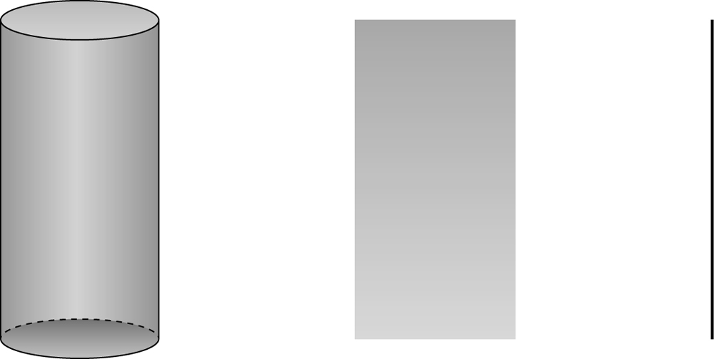
Fig. 2.2 A worldtube, worldsheet, and worldline, as generated by the time evolution of a disc, line (or open string), and point-particle respectively. Time goes up the page, and space across.

Still, much is missing in terms of representing a world like ours: we need to know more about what properties the basic objects have, how they combine and interact, and how (and why) they change and move. These require specifying the states and observables (roughly corresponding to kinematics) and their evolution over time (roughly corresponding to dynamics). This will supply us with a formal representation of a physical system (or possibly many systems, or even a whole universe or ensemble of such!). Referring back to the previous chapter, however, we find that this interpretative package (kinematics + dynamics) is rarely if ever uniquely determined by what we experience. For example, quantum theories can be supplied with radically different dynamics - e.g. ones in which measurement is central to the dynamics (causing the states to collapse to a definite value), and others in which measurement plays no such special role.

With such a representation to hand, we can ask all sorts of philosophical questions about the representation relation between model/theory and the world. For example, although it looks from the mathematical construction as though the spacetime points come first in ontological order, we should be careful in making such interpretive leaps. We can ask whether matter and spacetime are ‘equally fundamental,’ or if one is ‘more fundamental’ than the other. That is, if if we think our ultimate mathematical representation faithfully maps onto the world, we should be careful about confusing the order (or hierarchy) of construction of the representation with a corresponding order in reality, or in believing that every aspect of the mathematical structure has a corresponding target in the world.

There are other traps lying in wait that might be generated by the mathematical representation, yet without corresponding elements in reality. The modern version of the old pre-Socratic debate about the reality of space and time (and its relationship with matter) arises here. We can ask how symmetries of space and time act on physical situations and whether the new states they generate are physically real in this sense. We can ask whether spacetime points are real (despite the appearance of what are taken to be spacetime manifold points in the mathematical model). And so on. The point should be clear by now: mathematical representations of physical systems do not wear their interpretations on their sleeves - it will be even clearer by the end of this book …

In the next section we lay out the above-mentioned basic elements of a physical theory: <K>states, observables, dynamics<L>. This triple essentially packages together the ‘kinematics’ (states + observables: also relating to space, time, and motion) and the ‘dynamics’ (the physical forces and interactions constraining the kinematically possible motions), viewing a theory as the combination of these, thus making an interpreter’s life easier by giving us the systems and their properties along with a rule (the dynamics) for how they change and vary over time and space.

2.2 Kinematics and Dynamics

Space, time, and motion (of some basic objects) are the central elements in the kinematics of a physical theory. Usually, this basic background must be decided upon first, and then the laws (dynamics) will be introduced to constrain what motions are ‘actually possible’ relative to such a background. The division into kinematics and dynamics comes to us from Aristotle who viewed kinesis as a kind of ‘potential’ state of being while dynamics was an ‘actual’ state of being. Historians have wracked their brains over this distinction of Aristotle’s for many centuries, but translated into our terms we can see that kinematics concerns possible motions when we ignore the action of any forces and laws of nature in the spatiotemporal background, while dynamics concerns what motions can be actual once the laws (such as Newton’s laws of motion) are introduced. Mechanics is classically understood to be a fairly straightforward combination of these two components: kinematics + dynamics. All features of a world are understood to flow from a specification of both elements.

The kinematically possible trajectories will of course include the dynamically possible trajectories: the former space of possibilities is far larger than the latter. The modern distinction can be linked fairly closely to Aristotle’s (from the previous chapter) by focusing on what is possible in the two scenarios: kinematics is about which motions are possible given the constraints of the spacetime itself along with the barest features of the basic objects (so that, for example, in a world with three dimensions, motions requiring more dimensions will not be kinematically possible). We can think of these as metaphysically possible worlds, but not necessarily physically possible worlds: worlds that are conceivable, but are perhaps not compatible with our laws. Physical reasonableness is the province of dynamics, which narrows down the space of metaphysically possible worlds to a family of physically possible worlds: worlds that are compatible with our laws. We can think of the introduction of dynamics as a demand for explanation concerning why things change their motions (or stop): this demands forces (and we have the law of inertia, embodying the tendency of bodies to stay in motion unless forced to do otherwise). Hence, we have the standard conception of kinematics as the study of the motions of bodies in the absence of forces, and dynamics as the study of the effects of forces on those motions.

Though we utilize mathematics in this representation of trajectories (motions), especially using geometrical notions, there is a radical disconnect in how the physically applied concepts relate to the pure (mathematical) concepts. For example, a motion in the geometrical sense simply involves associating one point to another point, with no sense of a continuous trajectory linking them (at least not of necessity: one could imagine the point being carried along in a continuous path, but it is not essential). In the case of physical motions, however, the smooth paths between initial and final points are crucial, and form part of our picture of how the world works - not least because we often need to know the duration of the time interval during which some continuous path was traversed. But deeper than this (though not undeniable) is the belief that in order to get from a point A to a point B, the points in between must be traversed, during which the object that moves retains its identity in some sense (and so is the same object at B as it was at A - a relation sometimes called ‘genidentity’).

In modern approaches to physics, we do in fact shift to a more abstract representation: we speak of ‘states’ and ‘observables’ in place of kinematics (with its associated space, time, and motion). But we don’t fully dispense with space and motion; rather, a different kind of space and motion is employed, in the form of a state space and trajectories in this space. Just as we might build up a space from all possible combinations of some parameters, such as x, y, z measurements for ordinary space, we can also view the so-called ‘canonical variables’ as ‘generalized coordinates’ for this new kind of space (known as phase space: the state space of classical mechanics). Each point represents a different assignment of position and momentum to a system. This lets us do things we can’t do in ordinary physical space. For example, when we are dealing with a complex system of many particles (with a large number of particles, N), it would be a complicated task to deal individually with each of their paths through three-dimensional space. But with state spaces we can bundle all of this information into a new space of 6N-dimensions, in which a single point represents the positions (a ‘configuration’) and momenta of all N particles (taking into account each particle’s three spatial coordinates in ordinary space and their momenta in three spatial directions) taken at an instant of time.

Let us fill in some of the missing details from the above account. The state of a system, as the name suggests, is a snapshot of a system, containing complete information about it at an instant of time - the system itself is understood to be well represented by this state, which is essentially built from its properties. In classical mechanics this state is simply the position q (in ‘physical space’) of a particle together with its momentum p (the ‘canonical variables’ from above). The idea is that from such a specification of a state, we can run it through the laws of the theory to get to the system’s state at any other time (the dynamics in this new scheme). The state is, in this sense, the input (the programme) for the laws (the processor: a certain set of equations of motion known as Hamilton’s equations - basically, Newton’s laws of motion rewritten in fancier mathematics!), which separate the physically possible evolutions from the impossible ones.

Physics, at its most general, is concerned with physical quantities (in ordinary language we would call them ‘properties’), the interactions between quantities of the same and different kinds, and the rate of change of such quantities. Once we have our set of quantities, which we’ll label (i.e. the observables: the things we can measure), that will define the instantaneous state of the object that interests us (and, in a sense, is how an object is defined in physics), we can think about how these quantities (and so the state, and so the object) might change over time. We can set up equations of motion of the general form:

(2.1)

Finding how a system will evolve then simply amounts to finding the particular function, which results from the investigations of physicists. Integrating both sides of the equation, we can find future (and past) values of from its present value. (However, as we will see in Chapter 7, in quantum mechanics, as standardly interpreted, this framework only holds while the system is unobserved (between observations); measurement instead delivers a random value from a distribution of possible values, known as eigenvalues. In other words, there are two kinds of dynamics. Naturally, it would be better to make do with one, in terms of the number of elements in one’s world-picture, and such interpretations exist, as we will see.)

The position and momentum above are observables of the system, and we find that specifying all of the values of a system’s observables will uniquely determine its state - likewise, knowing the state means knowing the values of the observables. We measure observables to gain knowledge about the state. Hence, we have a perfect correlation between states and (complete sets) of observables at an instant t—(q(t), p(t)) are complete in classical mechanics in the sense that all other observables can be constructed from them using some mathematical operations. Such observables provide the core link between theory and world in the context of physics: they are the things we measure and whose values we predict. As such, they ground the qualitative character of a world: two worlds that are exact duplicates in terms of all of their observables will thereby be qualitatively indistinguishable (a feature that will be important in later examples). (The observables of classical mechanics have a dual role: on the one hand they are measurable quantities, allowing us to latch the theory onto the world, providing information about a state of the world. On the other hand they generate specific transitions of the state of a system from one to another: for example, the energy observable (aka the Hamiltonian function), when viewed in phase space terms, generates time-translations.)

Fig. 2.3 Representation of an observable in classical physics, mediating between an abstract state space and some numerical value that is associated with an experimental outcome n ∊ .

The observables in the classical case are functions from the phase space to (real) numbers: this is the link between the abstract representation, given by the state space, and reality, as given in measurements that can be associated with real number values. Take as an extremely simple example (a standard case study for physics introductions): a coin. This is a two-state system, and so it has a state space with just two points: Heads and Tails. An observable would have to be a function on this space, so that it spits out some numerical value depending on what state it is fed. We can write (Heads) = 1 and (Tails) = 0 - now we have made this association, if we want to be formal we can write the state space as = {0, 1}. Far more complicated examples occur in physics, such as energy observables that spit out a number representing the total energy of a system (that can deliver a continuum of possible values, rather than {0, 1}) when fed a point from the phase space. But still, this simple setup gets the basic point: classical observables are functions from the state space to numbers: : → (see fig. 2.3).

Quite naturally, the system’s state space will depend on the kind of system it is. Quantum mechanical systems are so radically different (e.g. not generally possessing sharp values for their observables, but instead a ‘spread’ of possible values called eigenvalues, which have probabilities assigned to them, or to their being found on measurement), however, that a different setup is required. The position and momentum observables that have real number values in the classical context are understood to be operators (‘Hermitian matrices’ in the jargon) on states in the quantum context. However, the eigenvalues of the operator (representing measurement outcomes) do have real number values, and these are what we measure in experiments (see fig. 2.4). These operators, as with the classical observables, also serve to create new states from old by their action.

As we will see later, much of this difference has to do with the fact that quantum particles have both wave and particle aspects. For this reason, the state of a system is represented by a function ψ(x, t) (a ‘wavefunction’) that represents the amplitude of the wave aspect of the system at the location x (given by three spatial coordinates) at time t. This wavefunction must be a complex number in order to represent the interference effects usually associated with wave phenomena and so is not itself an observable quantity. But one can construct a real-valued quantity that is observable by taking its squared modulus (the wave’s ‘intensity’): |ψ|² - this is the ‘complex square’ involving multiplication of the complex number by its complex conjugate: |ψ|² = ψ*(x, t)ψ(x, t). If you want to know the probability of finding a particle at some particular location x at time t, Prob(x, t), it is this squared modulus that you need to invoke. If we make the identification Prob(x, t) = |ψ|², then if all the possible outcomes for the location are integrated together (i.e. integrate over an interval, say from a to b), then, since probabilities must always sum to 1, we have:

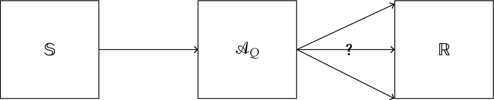
Fig. 2.4 Representation of an observable in quantum physics, mediating between an abstract state space and a range of numerical values (eigenvalues), each associated with a possible experimental outcome n_i ∊

(2.2)

For the dynamics, given in schematic form in eq. 2.1, in the case of quantum mechanics, we need an equation for the behavior of this wave-function ψ that is written as a function of ψ: this is the Schrödinger equation. The state space in which the various ψ are represented is known as ‘Hilbert space’ (a kind of vector space) in which states are represented by ‘rays’ (basically, vectors with some redundancy removed) in the space. This has the appropriate properties to represent the observed wavelike features of quantum systems. The observables (operators) are then understood to be objects that act on this space (simply: matrices acting on vectors) to produce numbers (the eigenvalues) comparable with experiment - these matrices must be Hermitian (self-adjoint, or equal to their own conjugates) precisely to get experimentally measurable real numbers out.

Hence, though there are very significant differences in the specific mathematical objects used to represent the states, observables, and dynamics, the same basic structures (harking back to the distinction between kinematics and dynamics) for representing the world and our engagement with it are utilized - ditto in statistical physics (which can be classical or quantum). However, we will find in later parts of this book that some pressure is placed on the ordering of the triple, ⟨(states, observables), dynamics⟩, since in general relativity the dynamics need to be solved first before sense can be made of the kinematics: spacetime geometry (needed for the definition of kinematics) comes out of solutions to the equations of motion (the dynamics) of general relativity - the slogan is ‘no kinematics without dynamics’.

2.3 Reference Frames, Invariance, and Covariance

In a great many cases, we can determine the basic features of a theory by invoking certain ‘principles’ on which the theory is based. Principles of physical theory are supposed to be claims about the world that are somehow more robust than most other such claims about the natural world. They say things about the world that are very hard to imagine not being true. In other words, they are as close to universal (empirical) truths as one can get in physical theories. Such principles are really ‘meta-laws’ (laws about laws). Special relativity, for example, involves two core principles:

SR1 All inertial frames are equal (from the point of view of mechanical and electromagnetic physical quantities and laws).

SR2 The speed of light is constant (in any and all inertial frames).

Or we have the single principle of Galilean relativity satisfied by non-relativistic laws:

G The laws of motion have the same form in all inertial frames (from the point of view of mechanical physical quantities and laws).

In the case of thermodynamics, one has:

T The laws should not allow the creation of perpetual motion machines.

These laws govern laws: if a theory is to describe specially relativistic systems then it must contain only laws that satisfy the two principles, SR1 and SR2, above. In a sense, the principles constitute what it is to be a specially relativistic (or Galilean relativistic or thermodynamic, and so on) system. While the ‘normal’ laws of a theory might involve a reference to some specific type of system (particular particles or fields, for example), these meta-laws float above such details: they are far more general, and therefore also more robust (i.e. to changes in the specific details of the theories that implement the principles). For example, special relativity was devised before quantum mechanics came about, yet it applies just as well in quantum mechanics as it does in classical physics.

Often, as seen above, these principles and laws concern the extent to which the reference frame, from which observations are made, is arbitrary. A reference frame can simply be understood to be a set of coordinates (x, y, z), which we can think of as a spatial frame in which measurements will be ‘recorded,’ and a time coordinate t, which we can think of as the reading of ‘clock time’ for these measurements. This is the laboratory of physics, though here it is presented rather abstractly.

Laboratories will usually vary between observers. For example, experiments performed on the international space station will occupy a different frame of reference to yours in your office or wherever you are reading this book. One can imagine other experiments taking place in a laboratory that is rotating (i.e. spinning on its own axis), which would involve a different reference frame. In order to make sense of these differences we need some way of relating them to one another, so that arbitrary features of the reference frame are not mistaken for features of reality. Transformation laws link the various reference frames, and allow us to see that the physical quantities that we measure do not depend on the frame in which they are measured: we extract the physical structure as that which is left invariant between the frames. As we see in the next chapter, these amount to symmetry principles.

These high-level laws are then defined by invariance with respect to some class of transformations (some way of shifting, rotating, evolving, twisting, or otherwise morphing the system), in which case we say that the laws in question are covariant with respect to those transformations - with the systems themselves then said to be invariant rather than covariant (the relevant quantities of the systems, such as energy or momentum, are then said to be conserved). In the case of special relativity above, the task was to find a set of transformation laws that preserve the principles (given that those principles seem to have a solid status in reality, as revealed by experiment). These are known as the Lorentz transformations, which Einstein encoded into the structure of spacetime (thus providing an entirely new kinematic framework for considering the motion of bodies in space and time). In the case of Newton’s equations of motion one has to find transformation laws that preserve those equations - these are the so-called Galilean transformations (discussed in the next chapter: for now, think of these, and the Lorentz transformations, simply as ways of moving a system around in space and time). We can, given this, rewrite the principles from above as:

G Galilean relativity → The covariance of the equations of motion (laws) under Galilean transformations.

SR Special relativity → The covariance of the equations of motion (laws) under Lorentz transformations.

These relativity principles bring into center stage the specific reference frames as characterized by their invariance under some specific set of transformations. It is the invariance that is really key. We turn to these invariances (symmetries) in the next chapter.

2.4 Further Readings

There are several books that I wish I’d known about when I really started becoming keen on physics. I hope these will prove useful for those wishing to build a solid background in mathematics and physics.

Fun

· Robert Mills (1994) Space, Time and Quanta. W. H. Freeman.
- Brilliant exposition of the basics of contemporary physics. For beginners, but manages to introduce many important mathematical concepts.

· John Taylor (2001) Hidden Unity in Nature’s Laws. Cambridge University Press.
- As above, elementary but written with a master’s touch.

Serious

· Leonard Susskind (2014) The Theoretical Minimum: What You Need to Know to Start Doing Physics. Basic Books.
- The perfect book for readers wishing to gain some facility in doing computations in physics.

· Lawrence Sklar (2013) Philosophy and the Foundations of Dynamics. Cambridge University Press.
- Textbook considering in depth philosophical aspects of many of the issues considered in this chapter - historical details are nicely interwoven with the philosophy.

Connoisseurs

· Roger Penrose (2007) The Road to Reality: A Complete Guide to the Laws of the Universe. Vintage.
- Do-it-yourself guide to becoming a theoretical physicist. It’s a fairly bumpy road, but full of philosophical insights and superb, readable introductions to even extremely difficult concepts.