Complexity: A Guided Tour - Melanie Mitchell (2009)

Part I. Background and History

Chapter 7. Defining and Measuring Complexity

THIS BOOK IS ABOUT COMPLEXITY, but so far I haven’t defined this term rigorously or given any clear way to answer questions such as these: Is a human brain more complex than an ant brain? Is the human genome more complex than the genome of yeast? Did complexity in biological organisms increase over the last four billion years of evolution? Intuitively, the answer to these questions would seem to be “of course.” However, it has been surprisingly difficult to come up with a universally accepted definition of complexity that can help answer these kinds of questions.

In 2004 I organized a panel discussion on complexity at the Santa Fe Institute’s annual Complex Systems Summer School. It was a special year: 2004 marked the twentieth anniversary of the founding of the institute. The panel consisted of some of the most prominent members of the SFI faculty, including Doyne Farmer, Jim Crutchfield, Stephanie Forrest, Eric Smith, John Miller, Alfred Hübler, and Bob Eisenstein—all well-known scientists in fields such as physics, computer science, biology, economics, and decision theory. The students at the school—young scientists at the graduate or postdoctoral level—were given the opportunity to ask any question of the panel. The first question was, “How do you define complexity?” Everyone on the panel laughed, because the question was at once so straightforward, so expected, and yet so difficult to answer. Each panel member then proceeded to give a different definition of the term. A few arguments even broke out between members of the faculty over their respective definitions. The students were a bit shocked and frustrated. If the faculty of the Santa Fe Institute—the most famous institution in the world devoted to research on complex systems—could not agree on what was meant by complexity, then how can there even begin to be a science of complexity?

The answer is that there is not yet a single science of complexity but rather several different sciences of complexity with different notions of what complexity means. Some of these notions are quite formal, and some are still very informal. If the sciences of complexity are to become a unified science of complexity, then people are going to have to figure out how these diverse notions—formal and informal—are related to one another, and how to most usefully refine the overly complex notion of complexity. This is work that largely remains to be done, perhaps by those shocked and frustrated students as they take over from the older generation of scientists.

I don’t think the students should have been shocked and frustrated. Any perusal of the history of science will show that the lack of a universally accepted definition of a central term is more common than not. Isaac Newton did not have a good definition of force, and in fact, was not happy about the concept since it seemed to require a kind of magical “action at a distance,” which was not allowed in mechanistic explanations of nature. While genetics is one of the largest and fastest growing fields of biology, geneticists still do not agree on precisely what the term gene refers to at the molecular level. Astronomers have discovered that about 95% of the universe is made up of “dark matter” and “dark energy” but have no clear idea what these two things actually consist of. Psychologists don’t have precise definitions for idea or concept, or know what these correspond to in the brain. These are just a few examples. Science often makes progress by inventing new terms to describe incompletely understood phenomena; these terms are gradually refined as the science matures and the phenomena become more completely understood. For example, physicists now understand all forces in nature to be combinations of four different kinds of fundamental forces: electromagnetic, strong, weak, and gravitational. Physicists have also theorized that the seeming “action at a distance” arises from the interaction of elementary particles. Developing a single theory that describes these four fundamental forces in terms of quantum mechanics remains one of the biggest open problems in all of physics. Perhaps in the future we will be able to isolate the different fundamental aspects of “complexity” and eventually unify all these aspects in some overall understanding of what we now call complex phenomena.

The physicist Seth Lloyd published a paper in 2001 proposing three different dimensions along which to measure the complexity of an object or process:

How hard is it to describe?

How hard is it to create?

What is its degree of organization?

Lloyd then listed about forty measures of complexity that had been proposed by different people, each of which addressed one or more of these three questions using concepts from dynamical systems, thermodynamics, information theory, and computation. Now that we have covered the background for these concepts, I can sketch some of these proposed definitions.

To illustrate these definitions, let’s use the example of comparing the complexity of the human genome with the yeast genome. The human genome contains approximately three billion base pairs (i.e., pairs of nucleotides). It has been estimated that humans have about 25,000 genes—that is, regions that code for proteins. Surprisingly, only about 2% of base pairs are actually parts of genes; the nongene parts of the genome are called noncoding regions. The noncoding regions have several functions: some of them help keep their chromosomes from falling apart; some help control the workings of actual genes; some may just be “junk” that doesn’t really serve any purpose, or has some function yet to be discovered.

I’m sure you’ve heard of the Human Genome project, but you may not know that there was also a Yeast Genome Project, in which the complete DNA sequences of several varieties of yeast were determined. The first variety that was sequenced turned out to have approximately twelve million base pairs and six thousand genes.

Complexity as Size

One simple measure of complexity is size. By this measure, humans are about 250 times as complex as yeast if we compare the number of base pairs, but only about four times as complex if we count genes.

Since 250 is a pretty big number, you may now be feeling rather complex, at least as compared with yeast. However, disappointingly, it turns out that the amoeba, another type of single-celled microorganism, has about 225 times as many base pairs as humans do, and a mustard plant called Arabidopsis has about the same number of genes that we do.

Humans are obviously more complex than amoebae or mustard plants, or at least I would like to think so. This means that genome size is not a very good measure of complexity; our complexity must come from something deeper than our absolute number of base pairs or genes (See figure 7.1).

Complexity as Entropy

Another proposed measure of the complexity of an object is simply its Shannon entropy, defined in chapter 3 to be the average information content or “amount of surprise” a message source has for a receiver. In our example, we could define a message to be one of the symbols A, C, G, or T. A highly ordered and very easy-to-describe sequence such as “A A A A A A A… A” has entropy equal to zero. A completely random sequence has the maximum possible entropy.

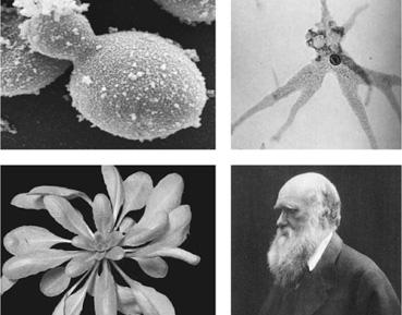
FIGURE 7.1. Clockwise from top left: Yeast, an amoeba, a human, and Arabidopsis. Which is the most complex? If you used genome length as the measure of complexity, then the amoeba would win hands down (if only it had hands). (Yeast photograph from NASA, [http://www.nasa.gov/mission_pages/station/science/experiments/Yeast-GAP.html]; amoeba photograph from NASA [http://ares.jsc.nasa.gov/astrobiology/biomarkers/_images/amoeba.jpg]; Arabidopsis photograph courtesy of Kirsten Bomblies; Darwin photograph reproduced with permission from John van Wyhe, ed., The Complete Work of Charles Darwin Online [http://darwin-online.org.uk/].)

There are a few problems with using Shannon entropy as a measure of complexity. First, the object or process in question has to be put in the form of “messages” of some kind, as we did above. This isn’t always easy or straightforward—how, for example, would we measure the entropy of the human brain? Second, the highest entropy is achieved by a random set of messages. We could make up an artificial genome by choosing a bunch of random As, Cs, Gs, and Ts. Using entropy as the measure of complexity, this random, almost certainly nonfunctional genome would be considered more complex than the human genome. Of course one of the things that makes humans complex, in the intuitive sense, is precisely that our genomes aren’t random but have been evolved over long periods to encode genes useful to our survival, such as the ones that control the development of eyes and muscles. The most complex entities are not the most ordered or random ones but somewhere in between. Simple Shannon entropy doesn’t capture our intuitive concept of complexity.

Complexity as Algorithmic Information Content

Many people have proposed alternatives to simple entropy as a measure of complexity. Most notably Andrey Kolmogorov, and independently both Gregory Chaitin and Ray Solomonoff, proposed that the complexity of an object is the size of the shortest computer program that could generate a complete description of the object. This is called the algorithmic information content of the object. For example, think of a very short (artificial) string of DNA:

ACACACACACACACACACAC (string 1).

A very short computer program, “Print A C ten times,” would spit out this pattern. Thus the string has low algorithmic information content. In contrast, here is a string I generated using a pseudo-random number generator:

ATCTGTCAAGACGGAACAT (string 2)

Assuming my random number generator is a good one, this string has no discernible overall pattern to it, and would require a longer program, namely “Print the exact string A T C T G T C A A A A C G G A A C A T.” The idea is that string 1 is compressible, but string 2 is not, so contains more algorithmic information. Like entropy, algorithmic information content assigns higher information content to random objects than ones we would intuitively consider to be complex.

The physicist Murray Gell-Mann proposed a related measure he called “effective complexity” that accords better with our intuitions about complexity. Gell-Mann proposed that any given entity is composed of a combination of regularity and randomness. For example, string 1 above has a very simple regularity: the repeating A C motif. String 2 has no regularities, since it was generated at random. In contrast, the DNA of a living organism has some regularities (e.g., important correlations among different parts of the genome) probably combined with some randomness (e.g., true junk DNA).

To calculate the effective complexity, first one figures out the best description of the regularities of the entity; the effective complexity is defined as the amount of information contained in that description, or equivalently, the algorithmic information content of the set of regularities.

String 1 above has the regularity that it is A C repeated over and over. The amount of information needed to describe this regularity is the algorithmic information content of this regularity: the length of the program “Print A C some number of times.” Thus, entities with very predictable structure have low effective complexity.

In the other extreme, string 2, being random, has no regularities. Thus there is no information needed to describe its regularities, and while the algorithmic information content of the string itself is maximal, the algorithmic information content of the string’s regularities—its effective complexity—is zero. In short, as we would wish, both very ordered and very random entities have low effective complexity.

The DNA of a viable organism, having many independent and interdependent regularities, would have high effective complexity because its regularities presumably require considerable information to describe.

The problem here, of course, is how do we figure out what the regularities are? And what happens if, for a given system, various observers do not agree on what the regularities are?

Gell-Mann makes an analogy with scientific theory formation, which is, in fact, a process of finding regularities about natural phenomena. For any given phenomenon, there are many possible theories that express its regularities, but clearly some theories—the simpler and more elegant ones—are better than others. Gell-Mann knows a lot about this kind of thing—he shared the 1969 Nobel prize in Physics for his wonderfully elegant theory that finally made sense of the (then) confusing mess of elementary particle types and their interactions.

In a similar way, given different proposed sets of regularities that fit an entity, we can determine which is best by using the test called Occam’s Razor. The best set of regularities is the smallest one that describes the entity in question and at the same time minimizes the remaining random component of that entity. For example, biologists today have found many regularities in the human genome, such as genes, regulatory interactions among genes, and so on, but these regularities still leave a lot of seemingly random aspects that don’t obey any regularities—namely, all that so-called junk DNA. If the Murray Gell-Mann of biology were to come along, he or she might find a better set of regularities that is simpler than that which biologists have so far identified and that is obeyed by more of the genome.

Effective complexity is a compelling idea, though like most of the proposed measures of complexity, it is hard to actually measure. Critics also have pointed out that the subjectivity of its definition remains a problem.

Complexity as Logical Depth

In order to get closer to our intuitions about complexity, in the early 1980s the mathematician Charles Bennett proposed the notion of logical depth. The logical depth of an object is a measure of how difficult that object is to construct. A highly ordered sequence of A, C, G, T (e.g., string 1, mentioned previously) is obviously easy to construct. Likewise, if I asked you to give me a random sequence of A, C, G, and T, that would be pretty easy for you to do, especially with the help of a coin you could flip or dice you could roll. But if I asked you to give me a DNA sequence that would produce a viable organism, you (or any biologist) would be very hard-pressed to do so without cheating by looking up already-sequenced genomes.

In Bennett’s words, “Logically deep objects… contain internal evidence of having been the result of a long computation or slow-to-simulate dynamical process, and could not plausibly have originated otherwise.” Or as Seth Lloyd says, “It is an appealing idea to identify the complexity of a thing with the amount of information processed in the most plausible method of its creation.”

To define logical depth more precisely, Bennett equated the construction of an object with the computation of a string of 0s and 1s encoding that object. For our example, we could assign to each nucleotide letter a two-digit code: A = 00, C = 01, G = 10, and T = 11. Using this code, we could turn any sequence of A, C, G, and T into a string of 0s and 1s. The logical depth is then defined as the number of steps that it would take for a properly programmed Turing machine, starting from a blank tape, to construct the desired sequence as its output.

Since, in general, there are different “properly programmed” Turing machines that could all produce the desired sequence in different amounts of time, Bennett had to specify which Turing machine should be used. He proposed that the shortest of these (i.e., the one with the least number of states and rules) should be chosen, in accordance with the above-mentioned Occam’s Razor.

Logical depth has very nice theoretical properties that match our intuitions, but it does not give a practical way of measuring the complexity of any natural object of interest, since there is typically no practical way of finding the smallest Turing machine that could have generated a given object, not to mention determining how long that machine would take to generate it. And this doesn’t even take into account the difficulty, in general, of describing a given object as a string of 0s and 1s.

Complexity as Thermodynamic Depth

In the late 1980s, Seth Lloyd and Heinz Pagels proposed a new measure of complexity, thermodynamic depth. Lloyd and Pagels’ intuition was similar to Bennett’s: more complex objects are harder to construct. However, instead of measuring the number of steps of the Turing machine needed to construct the description of an object, thermodynamic depth starts by determining “the most plausible scientifically determined sequence of events that lead to the thing itself,” and measures “the total amount of thermodynamic and informational resources required by the physical construction process.”

For example, to determine the thermodynamic depth of the human genome, we might start with the genome of the very first creature that ever lived and list all the evolutionary genetic events (random mutations, recombinations, gene duplications, etc.) that led to modern humans. Presumably, since humans evolved billions of years later than amoebas, their thermodynamic depth is much greater.

Like logical depth, thermodynamic depth is appealing in theory, but in practice has some problems as a method for measuring complexity. First, there is the assumption that we can, in practice, list all the events that lead to the creation of a particular object. Second, as pointed out by some critics, it’s not clear from Seth Lloyd and Heinz Pagels’ definition just how to define “an event.” Should a genetic mutation be considered a single event or a group of millions of events involving all the interactions between atoms and subatomic particles that cause the molecular-level event to occur? Should a genetic recombination between two ancestor organisms be considered a single event, or should we include all the microscale events that cause the two organisms to end up meeting, mating, and forming offspring? In more technical language, it’s not clear how to “coarse-grain” the states of the system—that is, how to determine what are the relevant macrostates when listing events.

Complexity as Computational Capacity

If complex systems—both natural and human-constructed—can perform computation, then we might want to measure their complexity in terms of the sophistication of what they can compute. The physicist Stephen Wolfram, for example, has proposed that systems are complex if their computational abilities are equivalent to those of a universal Turing machine. However, as Charles Bennett and others have argued, the ability to perform universal computation doesn’t mean that a system by itself is complex; rather, we should measure the complexity of the behavior of the system coupled with its inputs. For example, a universal Turing machine alone isn’t complex, but together with a machine code and input that produces a sophisticated computation, it creates complex behavior.

Statistical Complexity

Physicists Jim Crutchfield and Karl Young defined a different quantity, called statistical complexity, which measures the minimum amount of information about the past behavior of a system that is needed to optimally predict the statistical behavior of the system in the future. (The physicist Peter Grassberger independently defined a closely related concept called effective measure complexity.) Statistical complexity is related to Shannon’s entropy in that a system is thought of as a “message source” and its behavior is somehow quantified as discrete “messages.” Here, predicting the statistical behavior consists of constructing a model of the system, based on observations of the messages the system produces, such that the model’s behavior is statistically indistinguishable from the behavior of the system itself.

For example, a model of the message source of string 1 above could be very simple: “repeat A C”; thus its statistical complexity is low. However, in contrast to what could be done with entropy or algorithmic information content, a simple model could also be built of the message source that generates string 2: “choose at random from A, C, G, or T.” The latter is possible because models of statistical complexity are permitted to include random choices. The quantitative value of statistical complexity is the information content of the simplest such model that predicts the system’s behavior. Thus, like effective complexity, statistical complexity is low for both highly ordered and random systems, and is high for systems in between—those that we would intuitively consider to be complex.

Like the other measures described above, it is typically not easy to measure statistical complexity if the system in question does not have a ready interpretation as a message source. However, Crutchfield, Young, and their colleagues have actually measured the statistical complexity of a number of real-world phenomena, such as the atomic structure of complicated crystals and the firing patterns of neurons.

Complexity as Fractal Dimension

So far all the complexity measures I have discussed have been based on information or computation theoretic concepts. However, these are not the only possible sources of measures of complexity. Other people have proposed concepts from dynamical systems theory to measure the complexity of an object or process. One such measure is the fractal dimension of an object. To explain this measure, I must first explain what a fractal is.

The classic example of a fractal is a coastline. If you view a coastline from an airplane, it typically looks rugged rather than straight, with many inlets, bays, prominences, and peninsulas (Figure 7.2, top). If you then view the same coastline from your car on the coast highway, it still appears to have the exact same kind of ruggedness, but on a smaller scale (Figure 7.2, bottom). Ditto for the close-up view when you stand on the beach and even for the ultra close-up view of a snail as it crawls on individual rocks. The similarity of the shape of the coastline at different scales is called “self-similarity.”

The term fractal was coined by the French mathematician Benoit Mandelbrot, who was one of the first people to point out that the world is full of fractals—that is, many real-world objects have a rugged self-similar structure. Coastlines, mountain ranges, snowflakes, and trees are often-cited examples. Mandelbrot even proposed that the universe is fractal-like in terms of the distribution of galaxies, clusters of galaxies, clusters of clusters, et cetera. Figure 7.3 illustrates some examples of self-similarity in nature.

Although the term fractal is sometimes used to mean different things by different people, in general a fractal is a geometric shape that has “fine structure at every scale.” Many fractals of interest have the self-similarity property seen in the coastline example given above. The logistic-map bifurcation diagram from chapter 2 (figure 2.6) also has some degree of self-similarity; in fact the chaotic region of this (R greater than 3.57 or so) and many other systems are sometimes called fractal attractors.

Mandelbrot and other mathematicians have designed many different mathematical models of fractals in nature. One famous model is the so-called Koch curve (Koch, pronounced “Coke,” is the name of the Swedish mathematician who proposed this fractal). The Koch curve is created by repeated application of a rule, as follows.

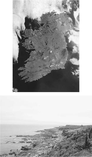
FIGURE 7.2. Top: Large-scale aerial view of Ireland, whose coastline has self-similar (fractal) properties. Bottom: Smaller-scale view of part of the Irish coastline. Its rugged structure at this scale resembles the rugged structure at the larger scale. (Top photograph from NASA Visible Earth [http://visibleearth.nasa.gov/]. Bottom photograph by Andreas Borchet, licensed under Creative Commons [http://creativecommons.org/licenses/by/3.0/].)

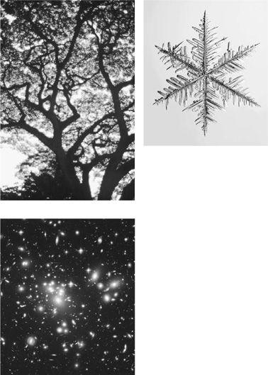
FIGURE 7.3. Other examples of fractal-like structures in nature: A tree, a snowflake (microscopically enlarged), a cluster of galaxies. (Tree photograph from the National Oceanic and Atmospheric Administration Photo Library. Snowflake photograph from [http://www.SnowCrystals.com], courtesy of Kenneth Libbrecht. Galaxy cluster photograph from NASA Space Telescope Science Institute.)

1. Start with a single line.

_______________________________

2. Apply the Koch curve rule: “For each line segment, replace its middle third by two sides of a triangle, each of length 1 / 3 of the original segment.” Here there is only one line segment; applying the rule to it yields:

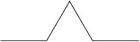
3. Apply the Koch curve rule to the resulting figure. Keep doing this forever. For example, here are the results from a second, third, and fourth application of the rule:

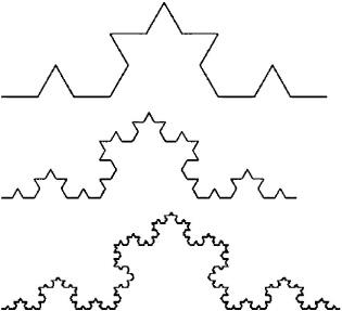
This last figure looks a bit like an idealized coastline. (In fact, if you turn the page 90 degrees to the left and squint really hard, it looks just like the west coast of Alaska.) Notice that it has true self-similarity: all of the subshapes, and their subshapes, and so on, have the same shape as the overall curve. If we applied the Koch curve rule an infinite number of times, the figure would be self-similar at an infinite number of scales—a perfect fractal. A real coastline of course does not have true self-similarity. If you look at a small section of the coastline, it does not have exactly the same shape as the entire coastline, but is visually similar in many ways (e.g., curved and rugged). Furthermore, in real-world objects, self-similarity does not go all the way to infinitely small scales. Real-world structures such as coastlines are often called “fractal” as a shorthand, but it is more accurate to call them “fractal-like,” especially if a mathematician is in hearing range.

Fractals wreak havoc with our familiar notion of spatial dimension. A line is one-dimensional, a surface is two-dimensional, and a solid is three-dimensional. What about the Koch curve?

First, let’s look at what exactly dimension means for regular geometric objects such as lines, squares, and cubes.

Start with our familiar line segment. Bisect it (i.e., cut it in half). Then bisect the resulting line segments, continuing at each level to bisect each line segment:

Each level is made up of two half-sized copies of the previous level.

Now start with a square. Bisect each side. Then bisect the sides of the resulting squares, continuing at each level to bisect every side:

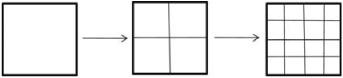
Each level is made up of four one-quarter-sized copies of the previous level.

Now, you guessed it, take a cube and bisect all the sides. Keep bisecting the sides of the resulting cubes:

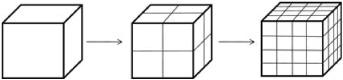
Each level is made up of eight one-eighth-sized copies of the previous level.

This sequence gives a meaning of the term dimension. In general, each level is made up of smaller copies of the previous level, where the number of copies is 2 raised to the power of the dimension (2^dimension). For the line, we get 2¹ = 2 copies at each level; for the square we get 2² = 4 copies at each level, and for the cube we get 2³ = 8 copies at each level. Similarly, if you trisect instead of bisect the lengths of the line segments at each level, then each level is made up of 3^dimension copies of the previous level. I’ll state this as a general formula:

Create a geometric structure from an original object by repeatedly dividing the length of its sides by a number x. Then each level is made up of x^dimension copies of the previous level.

Indeed, according to this definition of dimension, a line is one-dimensional, a square two-dimensional and a cube three-dimensional. All good and well.

Let’s apply an analogous definition to the object created by the Koch rule. At each level, the line segments of the object are three times smaller than before, and each level consists of four copies of the previous level. By our definition above, it must be true that 3^dimension is equal to 4. What is the dimension? To figure it out, I’ll do a calculation out of your sight (but detailed in the notes), and attest that according to our formula, the dimension is approximately 1.26. That is, the Koch curve is neither one- nor two-dimensional, but in between. Amazingly enough, fractal dimensions are not integers. That’s what makes fractals so strange.

In short, the fractal dimension quantifies the number of copies of a self-similar object at each level of magnification of that object. Equivalently, fractal dimension quantifies how the total size (or area, or volume) of an object will change as the magnification level changes. For example, if you measure the total length of the Koch curve each time the rule is applied, you will find that each time the length has increased by 4/3. Only perfect fractals—those whose levels of magnification extend to infinity—have precise fractal dimension. For real-world finite fractal-like objects such as coastlines, we can measure only an approximate fractal dimension.

I have seen many attempts at intuitive descriptions of what fractal dimension means. For example, it has been said that fractal dimension represents the “roughness,” “ruggedness,” “jaggedness,” or “complicatedness” of an object; an object’s degree of “fragmentation”; and how “dense the structure” of the object is. As an example, compare the coastline of Ireland (figure 7.2) with that of South Africa (figure 7.4). The former has higher fractal dimension than the latter.

One description I like a lot is the rather poetic notion that fractal dimension “quantifies the cascade of detail” in an object. That is, it quantifies how much detail you see at all scales as you dive deeper and deeper into the infinite cascade of self-similarity. For structures that aren’t fractals, such as a smooth round marble, if you keep looking at the structure with increasing magnification, eventually there is a level with no interesting details. Fractals, on the other hand, have interesting details at all levels, and fractal dimension in some sense quantifies how interesting that detail is as a function of how much magnification you have to do at each level to see it.

This is why people have been attracted to fractal dimension as a way of measuring complexity, and many scientists have applied this measure to real-world phenomena. However, ruggedness or cascades of detail are far from the only kind of complexity we would like to measure.

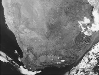
FIGURE 7.4. Coastline of South Africa. (Photograph from NASA Visible Earth [http://visibleearth.nasa.gov].)

Complexity as Degree of Hierarchy

In Herbert Simon’s famous 1962 paper “The Architecture of Complexity” Simon proposed that the complexity of a system can be characterized in terms of its degree of hierarchy: “the complex system being composed of subsystems that, in turn, have their own subsystems, and so on.” Simon was a distinguished political scientist, economist, and psychologist (among other things); in short, a brilliant polymath who probably deserves a chapter of his own in this book.

Simon proposed that the most important common attributes of complex systems are hierarchy and near-decomposibility. Simon lists a number of complex systems that are structured hierarchically—e.g., the body is composed of organs, which are in turn composed of cells, which are in turn composed of celluar subsystems, and so on. In a way, this notion is similar to fractals in the idea that there are self-similar patterns at all scales.

Near-decomposibility refers to the fact that, in hierarchical complex systems, there are many more strong interactions within a subsystem than between subsystems. As an example, each cell in a living organism has a metabolic network that consists of a huge number of interactions among substrates, many more than take place between two different cells.

Simon contends that evolution can design complex systems in nature only if they can be put together like building blocks—that is, only if they are hierachical and nearly decomposible; a cell can evolve and then become a building block for a higher-level organ, which itself can become a building block for an even higher-level organ, and so forth. Simon suggests that what the study of complex systems needs is “a theory of hierarchy.”

Many others have explored the notion of hierarchy as a possible way to measure complexity. As one example, the evolutionary biologist Daniel McShea, who has long been trying to make sense of the notion that the complexity of organisms increases over evolutionary time, has proposed a hierarchy scale that can be used to measure the degree of hierarchy of biological organisms. McShea’s scale is defined in terms of levels of nestedness: a higher-level entity contains as parts entities from the next lower level. McShea proposes the following biological example of nestedness:

Level 1: Prokaryotic cells (the simplest cells, such as bacteria)

Level 2: Aggregates of level 1 organisms, such as eukaryotic cells (more complex cells whose evolutionary ancestors originated from the fusion of prokaryotic cells)

Level 3: Aggregates of level 2 organisms, namely all multicellular organisms

Level 4: Aggregates of level 3 organisms, such as insect colonies and “colonial organisms” such as the Portuguese man o’ war.

Each level can be said to be more complex than the previous level, at least as far as nestedness goes. Of course, as McShea points out, nestedness only describes the structure of an organism, not any of its functions.

McShea used data both from fossils and modern organisms to show that the maximum hierarchy seen in organisms increases over evolutionary time. Thus this is one way in which complexity seems to have quantifiably increased with evolution, although measuring the degree of hierarchy in actual organisms can involve some subjectivity in determining what counts as a “part” or even a “level.”

There are many other measures of complexity that I don’t have space to cover here. Each of these measures captures something about our notion of complexity but all have both theoretical and practical limitations, and have so far rarely been useful for characterizing any real-world system. The diversity of measures that have been proposed indicates that the notions of complexity that we’re trying to get at have many different interacting dimensions and probably can’t be captured by a single measurement scale.