Chaos: Making a New Science - James Gleick (1988)

Strange Attractors

Big whorls have little whorls
Which feed on their velocity,
And little whorls have lesser whorls
And so on to viscosity.

—LEWIS F. RICHARDSON

TURBULENCE WAS A PROBLEM with pedigree. The great physicists all thought about it, formally or informally. A smooth flow breaks up into whorls and eddies. Wild patterns disrupt the boundary between fluid and solid. Energy drains rapidly from large-scale motions to small. Why? The best ideas came from mathematicians; for most physicists, turbulence was too dangerous to waste time on. It seemed almost unknowable. There was a story about the quantum theorist Werner Heisenberg, on his deathbed, declaring that he will have two questions for God: why relativity, and why turbulence. Heisenberg says, “I really think He may have an answer to the first question.”

Theoretical physics had reached a kind of standoff with the phenomenon of turbulence. In effect, science had drawn a line on the ground and said, Beyond this we cannot go. On the near side of the line, where fluids behave in orderly ways, there was plenty to work with. Fortunately, a smooth-flowing fluid does not act as though it has a nearly infinite number of independent molecules, each capable of independent motion. Instead, bits of fluid that start nearby tend to remain nearby, like horses in harness. Engineers have workable techniques for calculating flow, as long as it remains calm. They use a body of knowledge dating back to the nineteenth century, when understanding the motions of liquids and gases was a problem on the front lines of physics.

By the modern era, however, it was on the front lines no longer. To the deep theorists, fluid dynamics seemed to retain no mystery but the one that was unapproachable even in heaven. The practical side was so well understood that it could be left to the technicians. Fluid dynamics was no longer really part of physics, the physicists would say. It was mere engineering. Bright young physicists had better things to do. Fluid dynamicists were generally found in university engineering departments. A practical interest in turbulence has always been in the foreground, and the practical interest is usually one-sided: make the turbulence go away. In some applications, turbulence is desirable—inside a jet engine, for example, where efficient burning depends on rapid mixing. But in most, turbulence means disaster. Turbulent airflow over a wing destroys lift. Turbulent flow in an oil pipe creates stupefying drag. Vast amounts of government and corporate money are staked on the design of aircraft, turbine engines, propellers, submarine hulls, and other shapes that move through fluids. Researchers must worry about flow in blood vessels and heart valves. They worry about the shape and evolution of explosions. They worry about vortices and eddies, flames and shock waves. In theory the World War II atomic bomb project was a problem in nuclear physics. In reality the nuclear physics had been mostly solved before the project began, and the business that occupied the scientists assembled at Los Alamos was a problem in fluid dynamics.

What is turbulence then? It is a mess of disorder at all scales, small eddies within large ones. It is unstable. It is highly dissipative, meaning that turbulence drains energy and creates drag. It is motion turned random. But how does flow change from smooth to turbulent? Suppose you have a perfectly smooth pipe, with a perfectly even source of water, perfectly shielded from vibrations—how can such a flow create something random?

All the rules seem to break down. When flow is smooth, or laminar, small disturbances die out. But past the onset of turbulence, disturbances grow catastrophically. This onset—this transition—became a critical mystery in science. The channel below a rock in a stream becomes a whirling vortex that grows, splits off and spins downstream. A plume of cigarette smoke rises smoothly from an ashtray, accelerating until it passes a critical velocity and splinters into wild eddies. The onset of turbulence can be seen and measured in laboratory experiments; it can be tested for any new wing or propeller by experimental work in a wind tunnel; but its nature remains elusive. Traditionally, knowledge gained has always been special, not universal. Research by trial and error on the wing of a Boeing 707 aircraft contributes nothing to research by trial and error on the wing of an F-16 fighter. Even supercomputers are close to helpless in the face of irregular fluid motion.

Something shakes a fluid, exciting it. The fluid is viscous—sticky, so that energy drains out of it, and if you stopped shaking, the fluid would naturally come to rest. When you shake it, you add energy at low frequencies, or large wavelengths, and the first thing to notice is that the large wavelengths decompose into small ones. Eddies form, and smaller eddies within them, each dissipating the fluid’s energy and each producing a characteristic rhythm. In the 1930s A. N. Kolmogorov put forward a mathematical description that gave some feeling for how these eddies work. He imagined the whole cascade of energy down through smaller and smaller scales until finally a limit is reached, when the eddies become so tiny that the relatively larger effects of viscosity take over.

For the sake of a clean description, Kolmogorov imagined that these eddies fill the whole space of the fluid, making the fluid everywhere the same. This assumption, the assumption of homogeneity, turns out not to be true, and even Poincaré knew it forty years earlier, having seen at the rough surface of a river that the eddies always mix with regions of smooth flow. The vorticity is localized. Energy actually dissipates only in part of the space. At each scale, as you look closer at a turbulent eddy, new regions of calm come into view. Thus the assumption of homogeneity gives way to the assumption of intermittency. The intermittent picture, when idealized somewhat, looks highly fractal, with intermixed regions of roughness and smoothness on scales running down from the large to the small. This picture, too, turns out to fall somewhat short of the reality.

Closely related, but quite distinct, was the question of what happens when turbulence begins. How does a flow cross the boundary from smooth to turbulent? Before turbulence becomes fully developed, what intermediate stages might exist? For these questions, a slightly stronger theory existed. This orthodox paradigm came from Lev D. Landau, the great Russian scientist whose text on fluid dynamics remains a standard. The Landau picture is a piling up of competing rhythms. When more energy comes into a system, he conjectured, new frequencies begin one at a time, each incompatible with the last, as if a violin string responds to harder bowing by vibrating with a second, dissonant tone, and then a third, and a fourth, until the sound becomes an incomprehensible cacophony.

Any liquid or gas is a collection of individual bits, so many that they may as well be infinite. If each piece moved independently, then the fluid would have infinitely many possibilities, infinitely many “degrees of freedom” in the jargon, and the equations describing the motion would have to deal with infinitely many variables. But each particle does not move independently—its motion depends very much on the motion of its neighbors—and in a smooth flow, the degrees of freedom can be few. Potentially complex movements remain coupled together. Nearby bits remain nearby or drift apart in a smooth, linear way that produces neat lines in wind-tunnel pictures. The particles in a column of cigarette smoke rise as one, for a while.

Then confusion appears, a menagerie of mysterious wild motions. Sometimes these motions received names: the oscillatory, the skewed varicose, the cross-roll, the knot, the zigzag. In Landau’s view, these unstable new motions simply accumulated, one on top of another, creating rhythms with overlapping speeds and sizes. Conceptually, this orthodox idea of turbulence seemed to fit the facts, and if the theory was mathematically useless—which it was—well, so be it. Landau’s paradigm was a way of retaining dignity while throwing up the hands.

Water courses through a pipe, or around a cylinder, making a faint smooth hiss. In your mind, you turn up the pressure. A back-and-forth rhythm begins. Like a wave, it knocks slowly against the pipe. Turn the knob again. From somewhere, a second frequency enters, out of synchronization with the first. The rhythms overlap, compete, jar against one another. Already they create such a complicated motion, waves banging against the walls, interfering with one another, that you almost cannot follow it. Now turn up the knob again. A third frequency enters, then a fourth, a fifth, a sixth, all incommensurate. The flow has become extremely complicated. Perhaps this is turbulence. Physicists accepted this picture, but no one had any idea how to predict when an increase in energy would create a new frequency, or what the new frequency would be. No one had seen these mysteriously arriving frequencies in an experiment because, in fact, no one had ever tested Landau’s theory for the onset of turbulence.

THEORISTS CONDUCT EXPERIMENTS with their brains. Experimenters have to use their hands, too. Theorists are thinkers, experimenters are craftsmen. The theorist needs no accomplice. The experimenter has to muster graduate students, cajole machinists, flatter lab assistants. The theorist operates in a pristine place free of noise, of vibration, of dirt. The experimenter develops an intimacy with matter as a sculptor does with clay, battling it, shaping it, and engaging it. The theorist invents his companions, as a naive Romeo imagined his ideal Juliet. The experimenter’s lovers sweat, complain, and fart.

They need each other, but theorists and experimenters have allowed certain inequities to enter their relationships since the ancient days when every scientist was both. Though the best experimenters still have some of the theorist in them, the converse does not hold. Ultimately, prestige accumulates on the theorist’s side of the table. In high energy physics, especially, glory goes to the theorists, while experimenters have become highly specialized technicians, managing expensive and complicated equipment. In the decades since World War II, as physics came to be defined by the study of fundamental particles, the best publicized experiments were those carried out with particle accelerators. Spin, symmetry, color, flavor—these were the glamorous abstractions. To most laymen following science, and to more than a few scientists, the study of atomic particles was physics. But studying smaller particles, on shorter time scales, meant higher levels of energy. So the machinery needed for good experiments grew with the years, and the nature of experimentation changed for good in particle physics. The field was crowded, and the big experiment encouraged teams. The particle physics papers often stood out in Physical Review Letters: a typical authors list could take up nearly one-quarter of a paper’s length.

Some experimenters, however, preferred to work alone or in pairs. They worked with substances closer to hand. While such fields as hydrodynamics had lost status, solid-state physics had gained, eventually expanding its territory enough to require a more comprehensive name, “condensed matter physics”: the physics of stuff. In condensed matter physics, the machinery was simpler. The gap between theorist and experimenter remained narrower. Theorists expressed a little less snobbery, experimenters a little less defensiveness.

Even so, perspectives differed. It was fully in character for a theorist to interrupt an experimenter’s lecture to ask: Wouldn’t more data points be more convincing? Isn’t that graph a little messy? Shouldn’t those numbers extend up and down the scale for a few more orders of magnitude?

And in return, it was fully in character for Harry Swinney to draw himself up to his maximum height, something around five and a half feet, and say, “That’s true,” with a mixture of innate Louisiana charm and acquired New York irascibility. “That’s true if you have an infinite amount of noise-free data.” And wheel dismissively back toward the blackboard, adding, “In reality, of course, you have a limited amount of noisy data.”

Swinney was experimenting with stuff. For him the turning point had come when he was a graduate student at Johns Hopkins. The excitement of particle physics was palpable. The inspiring Murray Gell-Mann came to talk once, and Swinney was captivated. But when he looked into what graduate students did, he discovered that they were all writing computer programs or soldering spark chambers. It was then that he began talking to an older physicist starting to work on phase transitions—changes from solid to liquid, from nonmagnet to magnet, from conductor to superconductor. Before long Swinney had an empty room—not much bigger than a closet, but it was his alone. He had an equipment catalogue, and he began ordering. Soon he had a table and a laser and some refrigerating equipment and some probes. He designed an apparatus to measure how well carbon dioxide conducted heat around the critical point where it turned from vapor to liquid. Most people thought that the thermal conductivity would change slightly. Swinney found that it changed by a factor of 1,000. That was exciting—alone in a tiny room, discovering something that no one else knew. He saw the other-worldly light that shines from a vapor, any vapor, near the critical point, the light called “opalescence” because the soft scattering of rays gives the white glow of an opal.

Like so much of chaos itself, phase transitions involve a kind of macroscopic behavior that seems hard to predict by looking at the microscopic details. When a solid is heated, its molecules vibrate with the added energy. They push outward against their bonds and force the substance to expand. The more heat, the more expansion. Yet at a certain temperature and pressure, the change becomes sudden and discontinuous. A rope has been stretching; now it breaks. Crystalline form dissolves, and the molecules slide away from one another. They obey fluid laws that could not have been inferred from any aspect of the solid. The average atomic energy has barely changed, but the material—now a liquid, or a magnet, or a superconductor—has entered a new realm.

Günter Ahlers, at AT&T Bell Laboratories in New Jersey, had examined the so-called superfluid transition in liquid helium, in which, as temperature falls, the material becomes a sort of magical flowing liquid with no perceptible viscosity or friction. Others had studied superconductivity. Swinney had studied the critical point where matter changes between liquid and vapor. Swinney, Ahlers, Pierre Bergé, Jerry Gollub, Marzio Giglio—by the middle 1970s these experimenters and others in the United States, France, and Italy, all from the young tradition of exploring phase transitions, were looking for new problems. As intimately as a mail carrier learns the stoops and alleys of his neighborhood, they had learned the peculiar signposts of substances changing their fundamental state. They had studied a brink upon which matter stands poised.

The march of phase transition research had proceeded along stepping stones of analogy: a nonmagnet-magnet phase transition proved to be like a liquid-vapor phase transition. The fluid-superfluid phase transition proved to be like the conductor-superconductor phase transition. The mathematics of one experiment applied to many other experiments. By the 1970s the problem had been largely solved. A question, though, was how far the theory could be extended. What other changes in the world, when examined closely, would prove to be phase transitions?

It was neither the most original idea nor the most obvious to apply phase transition techniques to flow in fluids. Not the most original because the great hydrodynamic pioneers, Reynolds and Rayleigh and their followers in the early twentieth century, had already noted that a carefully controlled fluid experiment produces a change in the quality of motion—in mathematical terms a bifurcation. In a fluid cell, for example, liquid heated from the bottom suddenly goes from motionlessness to motion. Physicists were tempted to suppose that the physical character of that bifurcation resembled the changes in a substance that fell under the rubric of phase transitions.

It was not the most obvious sort of experiment because, unlike real phase transitions, these fluid bifurcations entailed no change in the substance itself. Instead they added a new element: motion. A still liquid becomes a flowing liquid. Why should the mathematics of such a change correspond to the mathematics of a condensing vapor?

IN 1973 SWINNEY was teaching at the City College of New York. Jerry Gollub, a serious and boyish graduate of Harvard, was teaching at Haverford. Haverford, a mildly bucolic liberal arts college near Philadelphia, seemed less than an ideal place for a physicist to end up. It had no graduate students to help with laboratory work and otherwise fill in the bottom half of the all-important mentor-protégé partnership. Gollub, though, loved teaching undergraduates and began building up the college’s physics department into a center widely known for the quality of its experimental work. That year, he took a sabbatical semester and came to New York to collaborate with Swinney.

With the analogy in mind between phase transitions and fluid instabilities, the two men decided to examine a classic system of liquid confined between two vertical cylinders. One cylinder rotated inside the other, pulling the liquid around with it. The system enclosed its flow between surfaces. Thus it restricted the possible motion of the liquid in space, unlike jets and wakes in open water. The rotating cylinders produced what was known as Couette-Taylor flow. Typically, the inner cylinder spins inside a stationary shell, as a matter of convenience. As the rotation begins and picks up speed, the first instability occurs: the liquid forms an elegant pattern resembling a stack of inner tubes at a service station. Doughnut-shaped bands appear around the cylinder, stacked one atop another. A speck in the fluid rotates not just east to west but also up and in and down and out around the doughnuts. This much was already understood. G. I. Taylor had seen it and measured it in 1923.

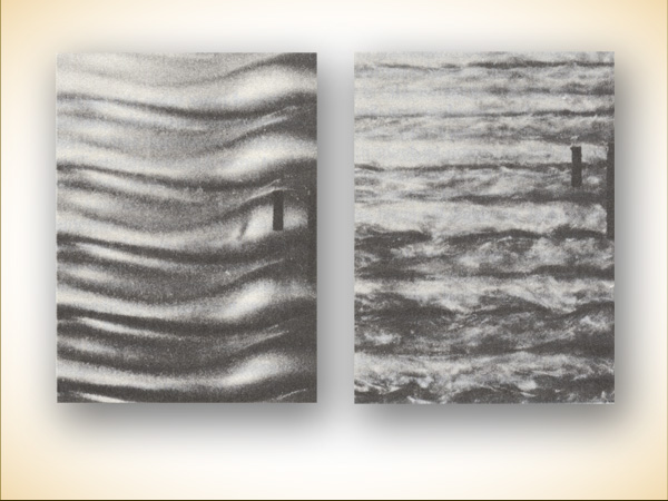
FLOW BETWEEN ROTATING CYLINDERS. The patterned flow of water between two cylinders gave Harry Swinney and Jerry Gollub a way to look at the onset of turbulence. As the rate of spin is increased, the structure grows more complex. First the water forms a characteristic pattern of flow resembling stacked doughnuts. Then the doughnuts begin to ripple. The physicists used a laser to measure the water’s changing velocity as each new instability appeared.

To study Couette flow, Swinney and Gollub built an apparatus that fit on a desktop, an outer glass cylinder the size of a skinny can of tennis balls, about a foot high and two inches across. An inner cylinder of steel slid neatly inside, leaving just one-eighth of an inch between for water. “It was a string-and-sealing-wax affair,” said Freeman Dyson, one of an unexpected series of prominent sightseers in the months that followed. “You had these two gentlemen in a poky little lab with essentially no money doing an absolutely beautiful experiment. It was the beginning of good quantitative work on turbulence.”

The two had in mind a legitimate scientific task that would have brought them a standard bit of recognition for their work and would then have been forgotten. Swinney and Gollub intended to confirm Landau’s idea for the onset of turbulence. The experimenters had no reason to doubt it. They knew that fluid dynamicists believed the Landau picture. As physicists they liked it because it fit the general picture of phase transitions, and Landau himself had provided the most workable early framework for studying phase transitions, based on his insight that such phenomena might obey universal laws, with regularities that overrode differences in particular substances. When Harry Swinney studied the liquid-vapor critical point in carbon dioxide, he did so with Landau’s conviction that his findings would carry over to the liquid-vapor critical point in xenon—and indeed they did. Why shouldn’t turbulence prove to be a steady accumulation of conflicting rhythms in a moving fluid?

Swinney and Gollub prepared to combat the messiness of moving fluids with an arsenal of neat experimental techniques built up over years of studying phase transitions in the most delicate of circumstances. They had laboratory styles and measuring equipment that a fluid dynamicist would never have imagined. To probe the rolling currents, they used laser light. A beam shining through the water would produce a deflection, or scattering, that could be measured in a technique called laser doppler interferometry. And the stream of data could be stored and processed by a computer—a device that in 1975 was rarely seen in a tabletop laboratory experiment.

Landau had said new frequencies would appear, one at a time, as a flow increased. “So we read that,” Swinney recalled, “and we said, fine, we will look at the transitions where these frequencies come in. So we looked, and sure enough there was a very well-defined transition. We went back and forth through the transition, bringing the rotation speed of the cylinder up and down. It was very well defined.”

When they began reporting results, Swinney and Gollub confronted a sociological boundary in science, between the domain of physics and the domain of fluid dynamics. The boundary had certain vivid characteristics. In particular, it determined which bureaucracy within the National Science Foundation controlled their financing. By the 1980s a Couette-Taylor experiment was physics again, but in 1973 it was just plain fluid dynamics, and for people who were accustomed to fluid dynamics, the first numbers coming out of this small City College laboratory were suspiciously clean. Fluid dynamicists just did not believe them. They were not accustomed to experiments in the precise style of phase-transition physics. Furthermore, in the perspective of fluid dynamics, the theoretical point of such an experiment was hard to see. The next time Swinney and Gollub tried to get National Science Foundation money, they were turned down. Some referees did not credit their results, and some said there was nothing new.

But the experiment had never stopped. “There was the transition, very well defined,” Swinney said. “So that was great. Then we went on, to look for the next one.”

There the expected Landau sequence broke down. Experiment failed to confirm theory. At the next transition the flow jumped all the way to a confused state with no distinguishable cycles at all. No new frequencies, no gradual buildup of complexity. “What we found was, it became chaotic.” A few months later, a lean, intensely charming Belgian appeared at the door to their laboratory.

DAVID RUELLE SOMETIMES SAID there were two kinds of physicists, the kind that grew up taking apart radios—this being an era before solid-state, when you could still look at wires and orange-glowing vacuum tubes and imagine something about the flow of electrons—and the kind that played with chemistry sets. Ruelle played with chemistry sets, or not quite sets in the later American sense, but chemicals, explosive or poisonous, cheerfully dispensed in his native northern Belgium by the local pharmacist and then mixed, stirred, heated, crystallized, and sometimes blown up by Ruelle himself. He was born in Ghent in 1935, the son of a gymnastics teacher and a university professor of linguistics, and though he made his career in an abstract realm of science he always had a taste for a dangerous side of nature that hid its surprises in cryptogamous fungoid mushrooms or saltpeter, sulfur, and charcoal.

It was in mathematical physics, though, that Ruelle made his lasting contribution to the exploration of chaos. By 1970 he had joined the Institut des Hautes Études Scientifiques, an institute outside Paris modeled on the Institute for Advanced Study in Princeton. He had already developed what became a lifelong habit of leaving the institute and his family periodically to take solitary walks, weeks long, carrying only a backpack through empty wildernesses in Iceland or rural Mexico. Often he saw no one. When he came across humans and accepted their hospitality—perhaps a meal of maize tortillas, with no fat, animal or vegetable—he felt that he was seeing the world as it existed two millennia before. When he returned to the institute he would begin his scientific existence again, his face just a little more gaunt, the skin stretched a little more tightly over his round brow and sharp chin. Ruelle had heard talks by Steve Smale about the horseshoe map and the chaotic possibilities of dynamical systems. He had also thought about fluid turbulence and the classic Landau picture. He suspected that these ideas were related—and contradictory.

Ruelle had no experience with fluid flows, but that did not discourage him any more than it had discouraged his many unsuccessful predecessors. “Always nonspecialists find the new things,” he said. “There is not a natural deep theory of turbulence. All the questions you can ask about turbulence are of a more general nature, and therefore accessible to nonspecialists.” It was easy to see why turbulence resisted analysis. The equations of fluid flow are nonlinear partial differential equations, unsolvable except in special cases. Yet Ruelle worked out an abstract alternative to Landau’s picture, couched in the language of Smale, with images of space as a pliable material to be squeezed, stretched, and folded into shapes like horseshoes. He wrote a paper at his institute with a visiting Dutch mathematician, Floris Takens, and they published it in 1971. The style was unmistakably mathematics—physicists, beware!—meaning that paragraphs would begin with Definition or Proposition or Proof, followed by the inevitable thrust: Let….

“Proposition (5.2). Let Xµ be a one-parameter family of C^k vectorfields on a Hilbert space H such that…”

Yet the title claimed a connection with the real world: “On the Nature of Turbulence,” a deliberate echo of Landau’s famous title, “On the Problem of Turbulence.” The clear purpose of Ruelle and Takens’s argument went beyond mathematics; they meant to offer a substitute for the traditional view of the onset of turbulence. Instead of a piling up of frequencies, leading to an infinitude of independent overlapping motions, they proposed that just three independent motions would produce the full complexity of turbulence. Mathematically speaking, some of their logic turned out to be obscure, wrong, borrowed, or all three—opinions still varied fifteen years later.

But the insight, the commentary, the marginalia, and the physics woven into the paper made it a lasting gift. Most seductive of all was an image that the authors called a strange attractor. This phrase was psychoanalytically “suggestive,” Ruelle felt later. Its status in the study of chaos was such that he and Takens jousted below a polite surface for the honor of having chosen the words. The truth was that neither quite remembered, but Takens, a tall, ruddy, fiercely Nordic man, might say, “Did you ever ask God whether he created this damned universe?…I don’t remember anything…. I often create without remembering it,” while Ruelle, the paper’s senior author, would remark softly, “Takens happened to be visiting IHES. Different people work differently. Some people would try to write a paper all by themselves so they keep all the credit.”

The strange attractor lives in phase space, one of the most powerful inventions of modern science. Phase space gives a way of turning numbers into pictures, abstracting every bit of essential information from a system of moving parts, mechanical or fluid, and making a flexible road map to all its possibilities. Physicists already worked with two simpler kinds of “attractors”: fixed points and limit cycles, representing behavior that reached a steady state or repeated itself continuously.

In phase space the complete state of knowledge about a dynamical system at a single instant in time collapses to a point. That point is the dynamical system—at that instant. At the next instant, though, the system will have changed, ever so slightly, and so the point moves. The history of the system time can be charted by the moving point, tracing its orbit through phase space with the passage of time.

How can all the information about a complicated system be stored in a point? If the system has only two variables, the answer is simple. It is straight from the Cartesian geometry taught in high school—one variable on the horizontal axis, the other on the vertical. If the system is a swinging, frictionless pendulum, one variable is position and the other velocity, and they change continuously, making a line of points that traces a loop, repeating itself forever, around and around. The same system with a higher energy level—swinging faster and farther—forms a loop in phase space similar to the first, but larger.

A little realism, in the form of friction, changes the picture. We do not need the equations of motion to know the destiny of a pendulum subject to friction. Every orbit must eventually end up at the same place, the center: position 0, velocity 0. This central fixed point “attracts” the orbits. Instead of looping around forever, they spiral inward. The friction dissipates the system’s energy, and in phase space the dissipation shows itself as a pull toward the center, from the outer regions of high energy to the inner regions of low energy. The attractor—the simplest kind possible—is like a pinpoint magnet embedded in a rubber sheet.

One advantage of thinking of states as points in space is that it makes change easier to watch. A system whose variables change continuously up or down becomes a moving point, like a fly moving around a room. If some combinations of variables never occur, then a scientist can simply imagine that part of the room as out of bounds. The fly never goes there. If a system behaves periodically, coming around to the same state again and again, then the fly moves in a loop, passing through the same position in phase space again and again. Phase-space portraits of physical systems exposed patterns of motion that were invisible otherwise, as an infrared landscape photograph can reveal patterns and details that exist just beyond the reach of perception. When a scientist looked at a phase portrait, he could use his imagination to think back to the system itself. This loop corresponds to that periodicity. This twist corresponds to that change. This empty void corresponds to that physical impossibility.

Even in two dimensions, phase-space portraits had many surprises in store, and even desktop computers could easily demonstrate some of them, turning equations into colorful moving trajectories. Some physicists began making movies and videotapes to show their colleagues, and some mathematicians in California published books with a series of green, blue, and red cartoon-style drawings—“chaos comics,” some of their colleagues said, with just a touch of malice. Two dimensions did not begin to cover the kinds of systems that physicists needed to study. They had to show more variables than two, and that meant more dimensions. Every piece of a dynamical system that can move independently is another variable, another degree of freedom. Every degree of freedom requires another dimension in phase space, to make sure that a single point contains enough information to determine the state of the system uniquely. The simple equations Robert May studied were one-dimensional—a single number was enough, a number that might stand for temperature or population, and that number defined the position of a point on a one-dimensional line. Lorenz’s stripped-down system of fluid convection was three-dimensional, not because the fluid moved through three dimensions, but because it took three distinct numbers to nail down the state of the fluid at any instant.

Spaces of four, five, or more dimensions tax the visual imagination of even the most agile topologist. But complex systems have many independent variables. Mathematicians had to accept the fact that systems with infinitely many degrees of freedom—untrammeled nature expressing itself in a turbulent waterfall or an unpredictable brain—required a phase space of infinite dimensions. But who could handle such a thing? It was a hydra, merciless and uncontrollable, and it was Landau’s image for turbulence: infinite modes, infinite degrees of freedom, infinite dimensions.

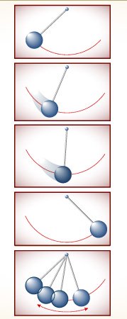
Velocity is zero as the pendulum starts its swing. Position is a negative number, the distance to the left of the center.

The two numbers specify a single point in two-dimensional phase space.

Velocity reaches its maximum as the pendulum’s position passes through zero.

Velocity declines again to zero, and then becomes negative to represent leftward motion.

ANOTHER WAY TO SEE A PENDULUM. One point in phase space (right) contains all the information about the state of a dynamical system at any instant (left). For a simple pendulum, two numbers—velocity and position—are all you need to know.

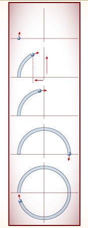
The points trace a trajectory that provides a way of visualizing the continuous long-term behavior of a dynamical system. A repeating loop represents a system that repeats itself at regular intervals forever.

If the repeating behavior is stable, as in a pendulum clock, then the system returns to this orbit after small perturbations. In phase space, trajectories near the orbit are drawn into it; the orbit is an attractor.

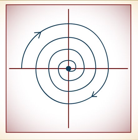
An attractor can be a single point. For a pendulum steadily losing energy to friction, all trajectories spiral inward toward a point that represents a steady state—in this case, the steady state of no motion at all.

A PHYSICIST HAD GOOD REASON to dislike a model that found so little clarity in nature. Using the nonlinear equations of fluid motion, the world’s fastest supercomputers were incapable of accurately tracking a turbulent flow of even a cubic centimeter for more than a few seconds. The blame for this was certainly nature’s more than Landau’s, but even so the Landau picture went against the grain. Absent any knowledge, a physicist might be permitted to suspect that some principle was evading discovery. The great quantum theorist Richard P. Feynman expressed this feeling. “It always bothers me that, according to the laws as we understand them today, it takes a computing machine an infinite number of logical operations to figure out what goes on in no matter how tiny a region of space, and no matter how tiny a region of time. How can all that be going on in that tiny space? Why should it take an infinite amount of logic to figure out what one tiny piece of space/time is going to do?”

Like so many of those who began studying chaos, David Ruelle suspected that the visible patterns in turbulent flow—self-entangled stream lines, spiral vortices, whorls that rise before the eye and vanish again—must reflect patterns explained by laws not yet discovered. In his mind, the dissipation of energy in a turbulent flow must still lead to a kind of contraction of the phase space, a pull toward an attractor. Certainly the attractor would not be a fixed point, because the flow would never come to rest. Energy was pouring into the system as well as draining out. What other kind of attractor could it be? According to dogma, only one other kind existed, a periodic attractor, or limit cycle—an orbit that attracted all other nearby orbits. If a pendulum gains energy from a spring while it loses it through friction—that is, if the pendulum is driven as well as damped—a stable orbit may be the closed loop in phase space that represents the regular swinging motion of a grandfather clock. No matter where the pendulum starts, it will settle into that one orbit. Or will it? For some initial conditions—those with the lowest energy—the pendulum will still settle to a stop, so the system actually has two attractors, one a closed loop and the other a fixed point. Each attractor has its “basin,” just as two nearby rivers have their own watershed regions.

In the short term any point in phase space can stand for a possible behavior of the dynamical system. In the long term the only possible behaviors are the attractors themselves. Other kinds of motion are transient. By definition, attractors had the important property of stability—in a real system, where moving parts are subject to bumps and jiggles from real-world noise, motion tends to return to the attractor. A bump may shove a trajectory away for a brief time, but the resulting transient motions die out. Even if the cat knocks into it, a pendulum clock does not switch to a sixty-two-second minute. Turbulence in a fluid was a behavior of a different order, never producing any single rhythm to the exclusion of others. A well-known characteristic of turbulence was that the whole broad spectrum of possible cycles was present at once. Turbulence is like white noise, or static. Could such a thing arise from a simple, deterministic system of equations?

Ruelle and Takens wondered whether some other kind of attractor could have the right set of properties. Stable—representing the final state of a dynamical system in a noisy world. Low-dimensional—an orbit in a phase space that might be a rectangle or a box, with just a few degrees of freedom. Nonperiodic—never repeating itself, and never falling into a steady grandfather-clock rhythm. Geometrically the question was a puzzle: What kind of orbit could be drawn in a limited space so that it would never repeat itself and never cross itself—because once a system returns to a state it has been in before, it thereafter must follow the same path. To produce every rhythm, the orbit would have to be an infinitely long line in a finite area. In other words—but the word had not been invented—it would have to be fractal.

By mathematical reasoning, Ruelle and Takens claimed that such a thing must exist. They had never seen one, and they did not draw one. But the claim was enough. Later, delivering a plenary address to the International Congress of Mathematicians in Warsaw, with the comfortable advantage of hindsight, Ruelle declared: “The reaction of the scientific public to our proposal was quite cold. In particular, the notion that continuous spectrum would be associated with a few degrees of freedom was viewed as heretical by many physicists.” But it was physicists—a handful, to be sure—who recognized the importance of the 1971 paper and went to work on its implications.

ACTUALLY, BY 1971 the scientific literature already contained one small line drawing of the unimaginable beast that Ruelle and Takens were trying to bring alive. Edward Lorenz had attached it to his 1963 paper on deterministic chaos, a picture with just two curves on the right, one inside the other, and five on the left. To plot just these seven loops required 500 successive calculations on the computer. A point moving along this trajectory in phase space, around the loops, illustrated the slow, chaotic rotation of a fluid as modeled by Lorenz’s three equations for convection. Because the system had three independent variables, this attractor lay in a three-dimensional phase space. Although Lorenz drew only a fragment of it, he could see more than he drew: a sort of double spiral, like a pair of butterfly wings interwoven with infinite dexterity. When the rising heat of his system pushed the fluid around in one direction, the trajectory stayed on the right wing; when the rolling motion stopped and reversed itself, the trajectory would swing across to the other wing.

The attractor was stable, low-dimensional, and nonperiodic. It could never intersect itself, because if it did, returning to a point already visited, from then on the motion would repeat itself in a periodic loop. That never happened—that was the beauty of the attractor. Those loops and spirals were infinitely deep, never quite joining, never intersecting. Yet they stayed inside a finite space, confined by a box. How could that be? How could infinitely many paths lie in a finite space?

In an era before Mandelbrot’s pictures of fractals had flooded the scientific marketplace, the details of constructing such a shape were hard to imagine, and Lorenz acknowledged an “apparent contradiction” in his tentative description. “It is difficult to reconcile the merging of two surfaces, one containing each spiral, with the inability of two trajectories to merge,” he wrote. But he saw an answer too delicate to appear in the few calculations within range of his computer. Where the spirals appear to join, the surfaces must divide, he realized, forming separate layers in the manner of a flaky mille-feuille. “We see that each surface is really a pair of surfaces, so that, where they appear to merge, there are really four surfaces. Continuing this process for another circuit, we see that there are really eight surfaces, etc., and we finally conclude that there is an infinite complex of surfaces, each extremely close to one or the other of two merging surfaces.” It was no wonder that meteorologists in 1963 left such speculation alone, nor that Ruelle a decade later felt astonishment and excitement when he finally learned of Lorenz’s work. He went to visit Lorenz once, in the years that followed, and left with a small sense of disappointment that they had not talked more of their common territory in science. With characteristic diffidence, Lorenz made the occasion a social one, and they went with their wives to an art museum.

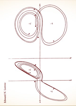
THE FIRST STRANGE ATTRACTOR. In 1963 Edward Lorenz could compute only the first few strands of the attractor for his simple system of equations. But he could see that the interleaving of the two spiral wings must have an extraordinary structure on invisibly small scales.

The effort to pursue the hints put forward by Ruelle and Takens took two paths. One was the theoretical struggle to visualize strange attractors. Was the Lorenz attractor typical? What other sorts of shapes were possible? The other was a line of experimental work meant to confirm or refute the highly unmathematical leap of faith that suggested the applicability of strange attractors to chaos in nature.

In Japan the study of electrical circuits that imitated the behavior of mechanical springs—but much faster—led Yoshisuke Ueda to discover an extraordinarily beautiful set of strange attractors. (He met an Eastern version of the coolness that greeted Ruelle: “Your result is no more than an almost periodic oscillation. Don’t form a selfish concept of steady states.”) In Germany Otto Rössler, a nonpracticing medical doctor who came to chaos by way of chemistry and theoretical biology, began with an odd ability to see strange attractors as philosophical objects, letting the mathematics follow along behind. Rössler’s name became attached to a particularly simple attractor in the shape of a band of ribbon with a fold in it, much studied because it was easy to draw, but he also visualized attractors in higher dimensions—“a sausage in a sausage in a sausage in a sausage,” he would say, “take it out, fold it, squeeze it, put it back.” Indeed, the folding and squeezing of space was a key to constructing strange attractors, and perhaps a key to the dynamics of the real systems that gave rise to them. Rössler felt that these shapes embodied a self-organizing principle in the world. He would imagine something like a wind sock on an airfield, “an open hose with a hole in the end, and the wind forces its way in,” he said. “Then the wind is trapped. Against its will, energy is doing something productive, like the devil in medieval history. The principle is that nature does something against its own will and, by self-entanglement, produces beauty.”

Making pictures of strange attractors was not a trivial matter. Typically, orbits would wind their ever-more-complicated paths through three dimensions or more, creating a dark scribble in space with an internal structure that could not be seen from the outside. To convert these three-dimensional skeins into flat pictures, scientists first used the technique of projection, in which a drawing represented the shadow that an attractor would cast on a surface. But with complicated strange attractors, projection just smears the detail into an indecipherable mess. A more revelatory technique was to make a return map, or a Poincaré map, in effect, taking a slice from the tangled heart of the attractor, removing a two-dimensional section just as a pathologist prepares a section of tissue for a microscope slide.

The Poincaré map removes a dimension from an attractor and turns a continuous line into a collection of points. In reducing an attractor to its Poincaré map, a scientist implicitly assumes that he can preserve much of the essential movement. He can imagine, for example, a strange attractor buzzing around before his eyes, its orbits carrying up and down, left and right, and to and fro through his computer screen. Each time the orbit passes through the screen, it leaves a glowing point at the place of intersection, and the points either form a random blotch or begin to trace some shape in phosphorus.

The process corresponds to sampling the state of a system every so often, instead of continuously. When to sample—where to take the slice from a strange attractor—is a question that gives an investigator some flexibility. The most informative interval might correspond to some physical feature of the dynamical system: for example, a Poincaré map could sample the velocity of a pendulum bob each time it passed through its lowest point. Or the investigator could choose some regular time interval, freezing successive states in the flash of an imaginary strobe light. Either way, such pictures finally began to reveal the fine fractal structure guessed at by Edward Lorenz.

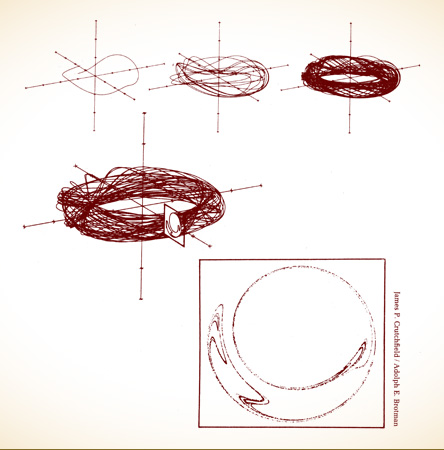
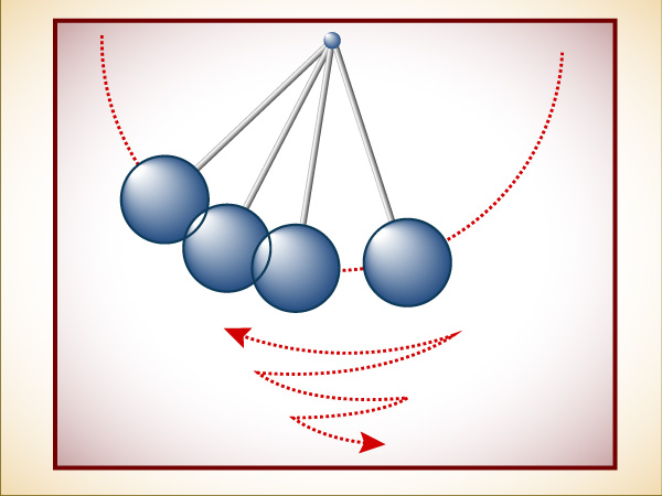
EXPOSING AN ATTRACTOR’S STRUCTURE. The strange attractor above—first one orbit, then ten, then one hundred—depicts the chaotic behavior of a rotor, a pendulum swinging through a full circle, driven by an energetic kick at regular intervals. By the time 1,000 orbits have been drawn (below), the attractor has become an impenetrably tangled skein.

To see the structure within, a computer can take a slice through an attractor, a so-called Poincaré section. The technique reduces a three-dimensional picture to two dimensions. Each time the trajectory passes through a plane, it marks a point, and gradually a minutely detailed pattern emerges. This example has more than 8,000 points, each standing for a full orbit around the attractor. In effect, the system is “sampled” at regular intervals. One kind of information is lost; another is brought out in high relief.

THE MOST ILLUMINATING STRANGE ATTRACTOR, because it was the simplest, came from a man far removed from the mysteries of turbulence and fluid dynamics. He was an astronomer, Michel Hénon of the Nice Observatory on the southern coast of France. In one way, of course, astronomy gave dynamical systems its start, the clockwork motions of planets providing Newton with his triumph and Laplace with his inspiration. But celestial mechanics differed from most earthly systems in a crucial respect. Systems that lose energy to friction are dissipative. Astronomical systems are not: they are conservative, or Hamiltonian. Actually, on a nearly infinitesimal scale, even astronomical systems suffer a kind of drag, with stars radiating away energy and tidal friction draining some momentum from orbiting bodies, but for practical purposes, astronomers’ calculations could ignore dissipation. And without dissipation, the phase space would not fold and contract in the way needed to produce an infinite fractal layering. A strange attractor could never arise. Could chaos?

Many astronomers have long and happy careers without giving dynamical systems a thought, but Hénon was different. He was born in Paris in 1931, a few years younger than Lorenz but, like him, a scientist with a certain unfulfilled attraction to mathematics. Hénon liked small, concrete problems that could be attached to physical situations—“not like the kind of mathematics people do today,” he would say. When computers reached a size suitable for hobbyists, Hénon got one, a Heathkit that he soldered together and played with at home. Long before that, though, he took on a particularly baffling problem in dynamics. It concerned globular clusters—crowded balls of stars, sometimes a million in one place, that form the oldest and possibly the most breathtaking objects in the night sky. Globular clusters are amazingly dense with stars. The problem of how they stay together and how they evolve over time has perplexed astronomers throughout the twentieth century.

Dynamically speaking, a globular cluster is a big many-body problem. The two-body problem is easy. Newton solved it completely. Each body—the earth and the moon, for example—travels in a perfect ellipse around the system’s joint center of gravity. Add just one more gravitational object, however, and everything changes. The three-body problem is hard, and worse than hard. As Poincaré discovered, it is most often impossible. The orbits can be calculated numerically for a while, and with powerful computers they can be tracked for a long while before uncertainties begin to take over. But the equations cannot be solved analytically, which means that long-term questions about a three-body system cannot be answered. Is the solar system stable? It certainly appears to be, in the short term, but even today no one knows for sure that some planetary orbits could not become more and more eccentric until the planets fly off from the system forever.

A system like a globular cluster is far too complex to be treated directly as a many-body problem, but its dynamics can be studied with the help of certain compromises. It is reasonable, for example, to think of individual stars winging their way through an average gravitational field with a particular gravitational center. Every so often, however, two stars will approach each other closely enough that their interaction must be treated separately. And astronomers realized that globular clusters generally must not be stable. Binary star systems tend to form inside them, stars pairing off in tight little orbits, and when a third star encounters a binary, one of the three tends to get a sharp kick. Every so often, a star will gain enough energy from such an interaction to reach escape velocity and depart the cluster forever; the rest of the cluster will then contract slightly. When Hénon took on this problem for his doctoral thesis in Paris in 1960, he made a rather arbitrary assumption: that as the cluster changed scale, it would remain self-similar. Working out the calculations, he reached an astonishing result. The core of a cluster would collapse, gaining kinetic energy and seeking a state of infinite density. This was hard to imagine, and furthermore it was not supported by the evidence of clusters so far observed. But slowly Hénon’s theory—later given the name “gravothermal collapse”—took hold.

Thus fortified, willing to try mathematics on old problems and willing to pursue unexpected results to their unlikely outcomes, he began work on a much easier problem in star dynamics.

This time, in 1962, visiting Princeton University, he had access for the first time to computers, just as Lorenz at M.I.T. was starting to use computers in meteorology. Hénon began modeling the orbits of stars around their galactic center. In reasonably simple form, galactic orbits can be treated like the orbits of planets around a sun, with one exception: the central gravity source is not a point, but a disk with thickness in three dimensions.

He made a compromise with the differential equations. “To have more freedom of experimentation,” as he put it, “we forget momentarily about the astronomical origin of the problem.” Although he did not say so at the time, “freedom of experimentation” meant, in part, freedom to play with the problem on a primitive computer. His machine had less than a thousandth of the memory on a single chip of a personal computer twenty-five years later, and it was slow, too. But like later experimenters in the phenomena of chaos, Hénon found that the oversimplification paid off. By abstracting only the essence of his system, he made discoveries that applied to other systems as well, and more important systems. Years later, galactic orbits were still a theoretical game, but the dynamics of such systems were under intense, expensive investigation by those interested in the orbits of particles in high-energy accelerators and those interested in the confinement of magnetic plasmas for the creation of nuclear fusion.

Stellar orbits in galaxies, on a time scale of some 200 million years, take on a three-dimensional character instead of making perfect ellipses. Three-dimensional orbits are as hard to visualize when the orbits are real as when they are imaginary constructions in phase space. So Hénon used a technique comparable to the making of Poincaré maps. He imagined a flat sheet placed upright on one side of the galaxy so that every orbit would sweep through it, as horses on a race track sweep across the finish line. Then he would mark the point where the orbit crossed this plane and trace the movement of the point from orbit to orbit.

Hénon had to plot these points by hand, but eventually the many scientists using this technique would watch them appear on a computer screen, like distant street lamps coming on one by one at nightfall. A typical orbit might begin with a point toward the lower left of the page. Then, on the next go-round, a point would appear a few inches to the right. Then another, more to the right and up a little—and so on. At first no pattern would be obvious, but after ten or twenty points an egg-shaped curve would take shape. The successive points actually make a circuit around the curve, but since they do not come around to exactly the same place, eventually, after hundreds or thousands of points, the curve is solidly outlined.

Such orbits are not completely regular, since they never exactly repeat themselves, but they are certainly predictable, and they are far from chaotic. Points never arrive inside the curve or outside it. Translated back to the full three-dimensional picture, the orbits were outlining a torus, or doughnut shape, and Hénon’s mapping was a cross-section of the torus. So far, he was merely illustrating what all his predecessors had taken for granted. Orbits were periodic. At the observatory in Copenhagen, from 1910 to 1930, a generation of astronomers painstakingly observed and calculated hundreds of such orbits—but they were only interested in the ones that proved periodic. “I, too, was convinced, like everyone else at that time, that all orbits should be regular like this,” Hénon said. But he and his graduate student at Princeton, Carl Heiles, continued computing different orbits, steadily increasing the level of energy in their abstract system. Soon they saw something utterly new.

First the egg-shaped curve twisted into something more complicated, crossing itself in figure eights and splitting apart into separate loops. Still, every orbit fell on some loop. Then, at even higher levels, another change occurred, quite abruptly. “Here comes the surprise,” Hénon and Heiles wrote. Some orbits became so unstable that the points would scatter randomly across the paper. In some places, curves could still be drawn; in others, no curve fit the points. The picture became quite dramatic: evidence of complete disorder mixed with the clear remnants of order, forming shapes that suggested “islands” and “chains of islands” to these astronomers. They tried two different computers and two different methods of integration, but the results were the same. They could only explore and speculate. Based solely on their numerical experimentation, they made a guess about the deep structure of such pictures. With greater magnification, they suggested, more islands would appear on smaller and smaller scales, perhaps all the way to infinity. Mathematical proof was needed—“but the mathematical approach to the problem does not seem too easy.”

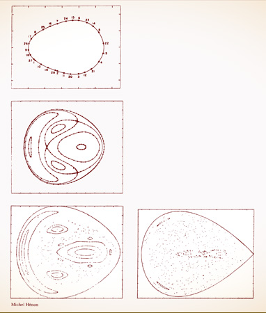
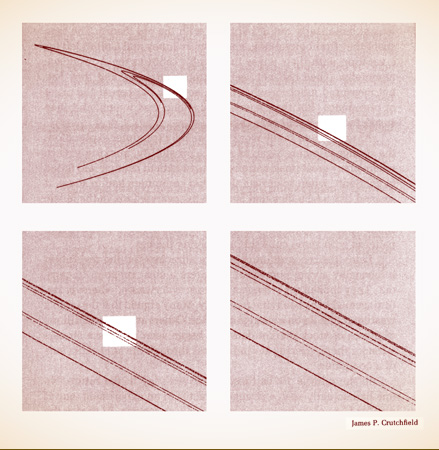
ORBITS AROUND THE GALACTIC CENTER. To understand the trajectories of the stars through a galaxy, Michel Hénon computed the intersections of an orbit with a plane. The resulting patterns depended on the system’s total energy. The points from a stable orbit gradually produced a continuous, connected curve (left). Other energy levels, however, produced complicated mixtures of stability and chaos, represented by regions of scattered points.

Hénon went on to other problems, but fourteen years later, when finally he heard about the strange attractors of David Ruelle and Edward Lorenz, he was prepared to listen. By 1976 he had moved to the Observatory of Nice, perched high above the Mediterranean Sea on the Grande Corniche, and he heard a talk by a visiting physicist about the Lorenz attractor. The physicist had been trying different techniques to illuminate the fine “micro-structure” of the attractor, with little success. Hénon, though dissipative systems were not his field (“sometimes astronomers are fearful of dissipative systems—they’re untidy”), thought he had an idea.

Once again, he decided to throw out all reference to the physical origins of the system and concentrate only on the geometrical essence he wanted to explore. Where Lorenz and others had stuck to differential equations—flows, with continuous changes in space and time—he turned to difference equations, discrete in time. The key, he believed, was the repeated stretching and folding of phase space in the manner of a pastry chef who rolls the dough, folds it, rolls it out again, folds it, creating a structure that will eventually be a sheaf of thin layers. Hénon drew a flat oval on a piece of paper. To stretch it, he picked a short numerical function that would move any point in the oval to a new point in a shape that was stretched upward in the center, an arch. This was a mapping—point by point, the entire oval was “mapped” onto the arch. Then he chose a second mapping, this time a contraction that would shrink the arch inward to make it narrower. And then a third mapping turned the narrow arch on its side, so that it would line up neatly with the original oval. The three mappings could be combined into a single function for purposes of calculation.

In spirit he was following Smale’s horseshoe idea. Numerically, the whole process was so simple that it could easily be tracked on a calculator. Any point has an x coordinate and a y coordinate to fix its horizontal and vertical position. To find the new x, the rule was to take the old y, add 1 and subtract 1.4 times the old x squared. To find the new y, multiply 0.3 by the old x. That is: x_new = y +1 - 1.4x² and y_new = 0.3x. Hénon picked a starting point more or less at random, took his calculator and started plotting new points, one after another, until he had plotted thousands. Then he used a real computer, an IBM 7040, and quickly plotted five million. Anyone with a personal computer and a graphics display could easily do the same.

At first the points appear to jump randomly around the screen. The effect is that of a Poincaré section of a three-dimensional attractor, weaving erratically back and forth across the display. But quickly a shape begins to emerge, an outline curved like a banana. The longer the program runs, the more detail appears. Parts of the outline seem to have some thickness, but then the thickness resolves itself into two distinct lines, then the two into four, one pair close together and one pair farther apart. On greater magnification, each of the four lines turns out to be composed of two more lines—and so on, ad infinitum. Like Lorenz’s attractor, Hénon’s displays infinite regress, like an unending sequence of Russian dolls one inside the other.

The nested detail, lines within lines, can be seen in final form in a series of pictures with progressively greater magnification. But the eerie effect of the strange attractor can be appreciated another way when the shape emerges in time, point by point. It appears like a ghost out of the mist. New points scatter so randomly across the screen that it seems incredible that any structure is there, let alone a structure so intricate and fine. Any two consecutive points are arbitrarily far apart, just like any two points initially nearby in a turbulent flow. Given any number of points, it is impossible to guess where the next will appear—except, of course, that it will be somewhere on the attractor.

The points wander so randomly, the pattern appears so ethereally, that it is hard to remember that the shape is an attractor. It is not just any trajectory of a dynamical system. It is the trajectory toward which all other trajectories converge. That is why the choice of starting conditions does not matter. As long as the starting point lies somewhere near the attractor, the next few points will converge to the attractor with great rapidity.

YEARS BEFORE, WHEN DAVID RUELLE arrived at the City College laboratory of Gollub and Swinney in 1974, the three physicists found themselves with a slender link between theory and experiment. One piece of mathematics, philosophically bold but technically uncertain. One cylinder of turbulent fluid, not much to look at, but clearly out of harmony with the old theory. The men spent the afternoon talking, and then Swinney and Gollub left for a vacation with their wives in Gollub’s cabin in the Adirondack mountains. They had not seen a strange attractor, and they had not measured much of what might actually happen at the onset of turbulence. But they knew that Landau was wrong, and they suspected that Ruelle was right.

THE ATTRACTOR OF HÉNON. A simple combination of folding and stretching produced an attractor that easy to compute yet still poorly understood by mathematicians. As thousands, the millions of points appear, more and more detail emerges. What appear to be single lines prove, on magnification, to be pairs, then pairs of pairs. Yet whether any two successive points appear nearby or far apart is unpredictable.

As an element in the world revealed by computer exploration, the strange attractor began as a mere possibility, marking a place where many great imaginations in the twentieth century had failed to go. Soon, when scientists saw what computers had to show, it seemed like a face they had been seeing everywhere, in the music of turbulent flows or in clouds scattered like veils across the sky. Nature was constrained. Disorder was channeled, it seemed, into patterns with some common underlying theme.

Later, the recognition of strange attractors fed the revolution in chaos by giving numerical explorers a clear program to carry out. They looked for strange attractors everywhere, wherever nature seemed to be behaving randomly. Many argued that the earth’s weather might lie on a strange attractor. Others assembled millions of pieces of stock market data and began searching for a strange attractor there, peering at randomness through the adjustable lens of a computer.

In the middle 1970s these discoveries lay in the future. No one had actually seen a strange attractor in an experiment, and it was far from clear how to go about looking for one. In theory the strange attractor could give mathematical substance to fundamental new properties of chaos. Sensitive dependence on initial conditions was one. “Mixing” was another, in a sense that would be meaningful to a jet engine designer, for example, concerned about the efficient combination of fuel and oxygen. But no one knew how to measure these properties, how to attach numbers to them. Strange attractors seemed fractal, implying that their true dimension was fractional, but no one knew how to measure the dimension or how to apply such a measurement in the context of engineering problems.

Most important, no one knew whether strange attractors would say anything about the deepest problem with nonlinear systems. Unlike linear systems, easily calculated and easily classified, nonlinear systems still seemed, in their essence, beyond classification—each different from every other. Scientists might begin to suspect that they shared common properties, but when it came time to make measurements and perform calculations, each nonlinear system was a world unto itself. Understanding one seemed to offer no help in understanding the next. An attractor like Lorenz’s illustrated the stability and the hidden structure of a system that otherwise seemed patternless, but how did this peculiar double spiral help researchers exploring unrelated systems? No one knew.

For now, the excitement went beyond pure science. Scientists who saw these shapes allowed themselves to forget momentarily the rules of scientific discourse. Ruelle, for example: “I have not spoken of the esthetic appeal of strange attractors. These systems of curves, these clouds of points suggest sometimes fireworks or galaxies, sometimes strange and disquieting vegetal proliferations. A realm lies there of forms to explore, and harmonies to discover.”