BioBuilder: Synthetic Biology in the Lab (2015)

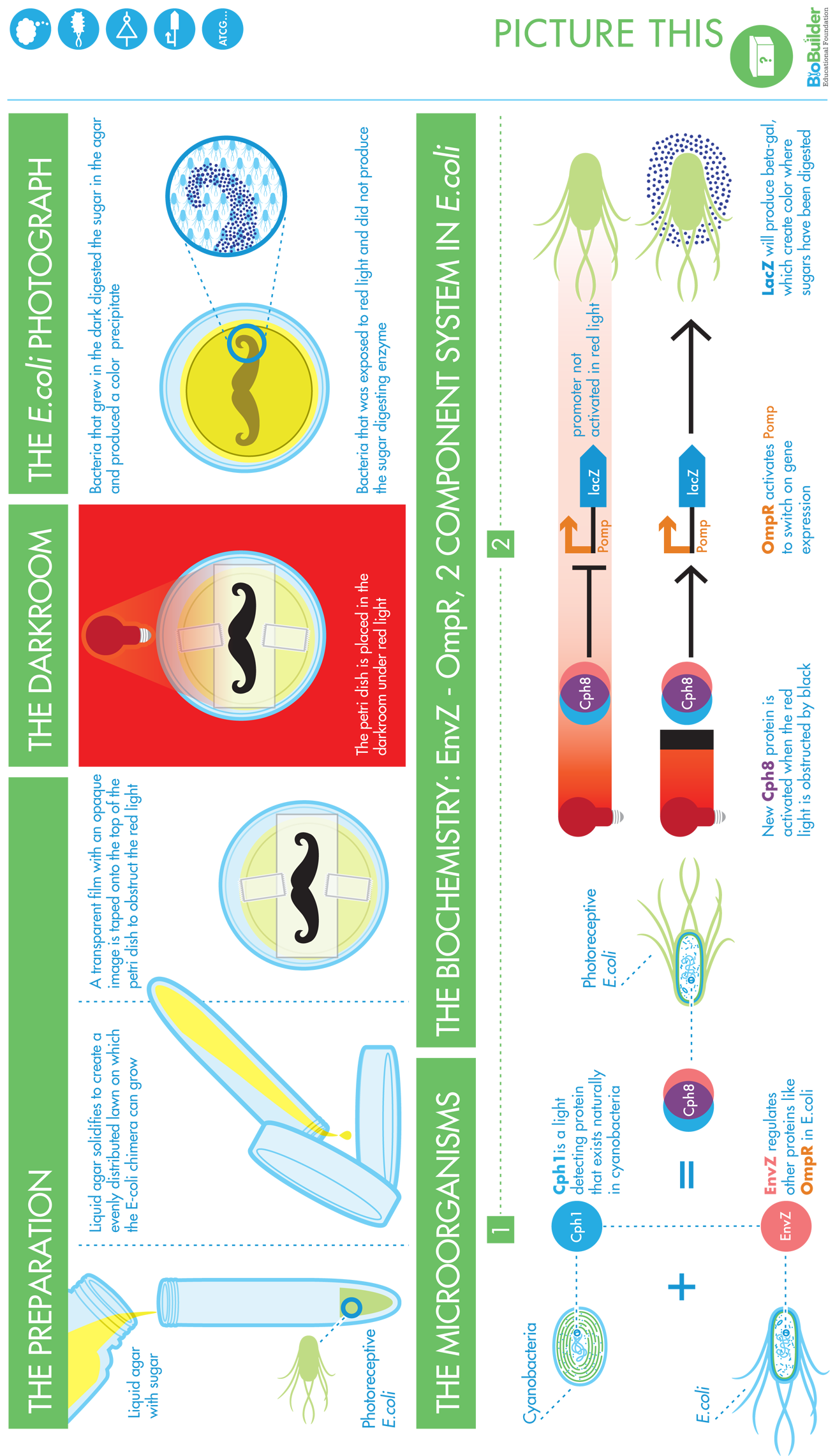
BioBuilder’s Picture This activity emphasizes the “design” phase of the design-build-test cycle. Picture This uses a system developed by a 2004 International Genetically Engineered Machines (iGEM) team that changes E. coli’s sensitivity to light, making the strain useful for “bacterial photography.” The team modified the cells to be both light-sensitive and color-producing, and it connected these genetic functions to each other (Figure 8-1). A lawn composed of these cells is able to reproduce an image printed on a mask by acting as photographic pixels, turning the cells’ color-generating genetic circuitry “on” in the dark or “off” in the light.

It took a lot of trial and error as well as a healthy dose of good luck for the iGEM team to successfully design and build the sophisticated genetic circuit that produced this photographic behavior. In the future, as synthetic biologists design even more sophisticated or complex living systems, they will need to rely on a crucial tool that other engineering disciplines have at their disposal: mathematical and physical modeling. When reliable modeling tools are available, synthetic biologists will be able to conduct computational simulations and experiments to test their systems before they begin working with the actual cells and DNA. Instead of starting a project by building the living system, they’ll gather information from models to anticipate some of the cell’s behaviors, which will help these synthetic biologists to make design choices. These models might not completely represent how the real system would behave—they’re only models, after all—but they should provide a powerful starting point and an excellent tool to ask questions that would be difficult or time consuming to explore in other ways. There is an important place in the field of synthetic biology for computer programmers and mathematical modelers to develop these simulation tools.

Figure 8-1. Bacterial photography system-level design. The bacterial photography system takes light as an input and produces color pixels as the output.

In BioBuilder’s Picture This activity, you can build two kinds of models for the bacterial photography system: a computational model and an electronic model. In practice, engineers would build models before building the actual system, but here, we work in reverse order. This way, we can reveal the general utility of building models in the first place. There are strengths and weaknesses to both models, as you’ll see, but each can provide valuable insight into the genetic system’s behavior. In this chapter, we first consider different types of models, including their benefits and drawbacks. Then we look at the iGEM team’s bacterial photography system in more detail.

Introduction to Modeling

It can take an architect many months, or even years, of careful planning to design a skyscraper so that it takes the right form and is structurally sound. During that time, the architect’s design process will include a variety of modeling approaches, some to help visualize what the building will look like when it’s complete, and others to anticipate how it will behave. These models are an investment that can save time and money if they are built before the skyscraper itself.

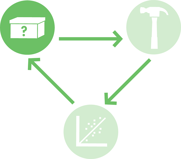
What kinds of models should you use? Depending on the nature of the project, architects might draw a two-dimensional blueprint, build a three-dimensional miniature model using balsa wood, or run a computer simulation (Figure 8-3) to test how a structure might respond to an earthquake. Each of these models has different strengths. For example, a balsa wood model can help a designer evaluate the aesthetics of the building, and a computer model could confirm that the building will not fail in a natural disaster. By using a variety of modeling techniques, it’s possible to rapidly consider different design options until one is found that meets the architect’s specifications and needs. In this way, modeling can help drive the design process before the building phase begins (Figure 8-2).

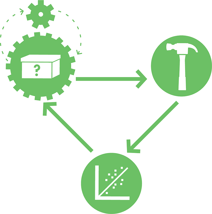
Figure 8-2. Illustrating the role of modeling in the design-build-test cycle. Modeling, symbolically depicted here as the small gear in the top left, can help drive the design process.

Figure 8-3. Some types of models. Models can take many different forms. Using our architecture example, a few useful models include blueprints (left), three-dimensional physical models (middle), and computational models (right).

Of course, no model, or even collection of models, can fully capture all aspects of the final design. Everyone who uses modeling techniques, be they architects or synthetic biologists, must work within the limits of each model. In most cases, people use a combination of different modeling techniques to form a relatively complete idea of how their system is likely to behave. But, using more models doesn’t automatically generate better data, because not all models are good models. Using an inappropriate computational model or building a physical model that misrepresents the system can send the work in the wrong direction. It’s crucial to understand how a model is made to properly interpret the results it provides.

Computational Modeling

Computational modeling (Figure 8-4) refers to the use of a computer to simulate the behavior of a particular design. To build computational models for synthetic biology, engineers input information about the individual components of their biological systems, including equations and algorithms that the computer can use to calculate the system’s expected behavior when all the components are put together in a cell. These equations might closely approximate the actual behavior of a biological system but are unlikely to reproduce it perfectly. For example, many equations that describe the speed and extent of reactions were first derived by scientists who were studying individual enzymes in isolation in test tubes, which is a much simpler context than the complex environment of a cell. In a cell, multiple enzymes can compete for the same reactant, or one enzyme’s product might inhibit another enzyme’s activity. In truth, we do not yet fully understand why our equations cannot fully capture cellular behavior, but we can make certain assumptions about molecular behaviors to approximate different conditions. For instance, the model might simplify the reaction rates so that they are all constant; thus, the model applies in some but not all cases.

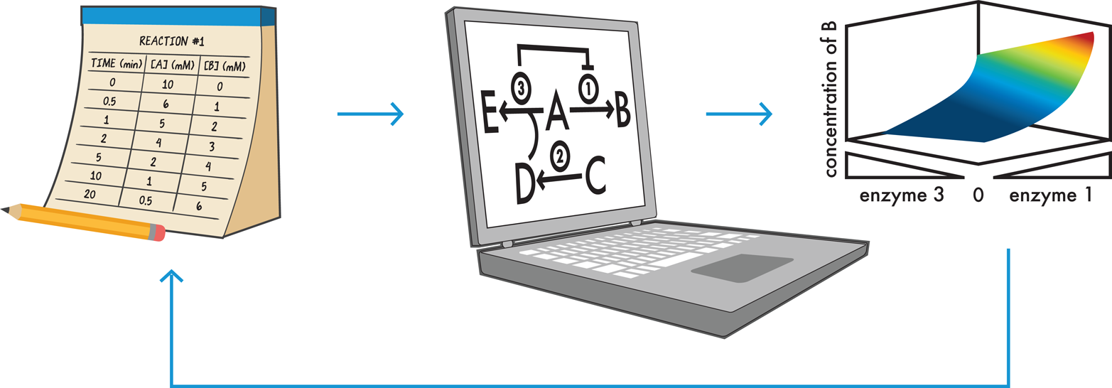
Figure 8-4. Computationally modeling cellular processes. Data (left) can be collected for each relevant reaction and integrated by a computer (center) to build a working model of the cell’s behavior and predict how the concentrations of different compounds will change over time (right). If the model’s output does not match the design specifications, the model can be adjusted or more data can be collected as appropriate and the simulation can be rerun as many times as is needed. In this way, computational modeling is a rapid way to “test” a design.

Despite their limitations, computational models are useful because they quickly and precisely solve equations that integrate multiple processes. The model’s output might not perfectly reflect nature, but even the model’s imperfections can teach us something new about the system with which we’re working. By building a computational model, we’re actually testing the limits of our understanding and maybe discovering important new aspects of the system that need to be incorporated into the model for it to reflect what’s observable.

Another benefit of computational models is that they can simulate the behavior of complex systems when the systems are exposed to a wide variety of conditions. Using a set of starting conditions, a computational model can calculate how the state of the system will change over time. Returning to the architecture example, a simulation could be used to determine how a building might respond to high winds. Inputs to the model might include factors such as steel strength, its response to temperature changes, and the anticipated wind speeds in the region. The architect could run simulations with different skyscraper heights, wind speeds (as shown in Figure 8-5), or building materials. A good computational model would adequately anticipate the behavior of different design options and help the architect determine the physical limits for the design.

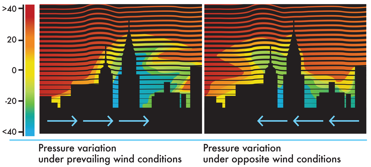
Figure 8-5. Modeling wind’s effect on pressure around a building. A computational model can predict how pressure will vary under prevailing wind conditions (left) and opposite wind conditions (right), with red indicating high wind pressure and blue low pressure.

A model draws information from two basic sources: its built-in knowledge base, and new information entered by the user. For example, an architect’s modeling software will likely contain information about how a variety of materials respond to different temperatures or wind speeds. This kind of common information is already built into the model. The architect using the model can then specify the type of steel to use and then run a simulation, sometimes called a modeling experiment, to see if it’s strong enough. Should the results indicate that the steel is not sufficient, it’s easy to run another simulation, inputting the information for a different type of steel. This approach, called computer-aided design (CAD), is obviously more efficient—and safer—than building an entire skyscraper, finding it’s not strong enough to withstand the winds, and being forced to rebuild.

Synthetic biology projects also benefit from computational modeling. Researchers have modeled a variety of cellular systems, with varying degrees of success depending on the sophistication, strengths, and weaknesses of the models. Just as an architect’s model contains built-in information for how specific materials respond to wind, computational models of biological systems include information about the dynamic behavior of proteins and other biomolecules. The more specific and accurate the information for each component of the system is, the better will be the resulting model. This is one reason why synthetic biologists measure the behavior of individual parts and are developing ways to share the information with one another via standardized data sheets, as introduced in the iTune Device chapter. As individual parts are better characterized experimentally, the resulting information can be included in models to improve their accuracy and biological relevance.

After a model is built and a simulation (or two or three) is run, it’s time to turn from the computer back to the laboratory bench. We can compare the results of the “wet lab” experiments to those from computational simulations, and then, ideally, the results are used to refine the computational model further. Through the combined and iterative approach of computational and bench work, they both improve, in spite of the limitations and assumptions intrinsic to each.

Physical Modeling

A complement to computational modeling is physical modeling. For example, an architect might create a miniature physical structure to help visualize a building project beyond what a computer simulation could reveal. For cells, which are microscopic, it’s unclear what a physical model might reveal. Consequently, synthetic biologists generally don’t build structural models to illustrate what their living systems would actually look like. However, a physical model of the information flow through a living system can be a benefit.

We can use electronic components to meet this end because they provide tangible and well-understood physical models that can illustrate and explore the design and the function of genetic circuits. Synthetic biologists have already applied terminology and logic principles from the mature fields of mechanical and electrical engineering to the design process for living systems, which is explored in the Fundamentals of Biodesign chapter. Electrical components also provide a useful tool for physically modeling genetic systems.

An electrical model for a biological system has a number of benefits, the most dramatic of which is the speed with which electrical engineers can create prototypes of a system. Engineers can build and test electrical systems quickly, taking only as long as is needed to correctly connect the wires, resistors, and other electronic components appropriately. By comparison, building a biological system is time-consuming and its outcome is less certain. Moreover, when it doesn’t work, the troubleshooting process can be very slow. In biology, there are no error messages that the cell gives (other than a failure to grow!) and no handy voltmeter or other measurement device to assess the proper functioning of individual modules within a system. Finally, the biological modules themselves are not, for the most part, made of standardized off-the-shelf parts that are available everywhere and that work every time. Electronics, which are not subject to any of these complications, can therefore provide excellent tangible representations of genetic circuits and biological systems for testing and troubleshooting. This type of physical model can help designers develop a deeper understanding of the system they are building and perhaps identify problems that were not apparent in other representations.

Of course, there are some ways in which electronic models fall short of adequately representing the circuitry of the system. Figure 8-6 illustrates that one limitation is the digital behavior of electronics—components are either “on” or “off.” Biological components, on the other hand, tend to behave in an analog fashion, with a range of behaviors between fully “on” and fully “off.”

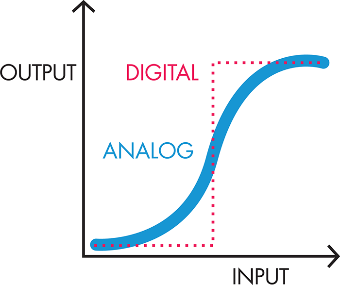
Figure 8-6. Digital versus analog signals. Digital signals show distinct on/off behavior (red dotted line). Low input does not generate any output. When the input passes a certain threshold, the output jumps to its maximum value. Analog signals, on the other hand, show a more gradual transition between off and on (blue solid line). As a result, input below the digital threshold can still generate some output, and input above the digital threshold can generate output less than the maximum value, even if the completely “off” and completely “on” values for both the digital and analog components are the same.

There’s a need for both digital and analog behaviors. For example, digital electronic behavior is like the light switch that turns a light bulb on or off, whereas analog behavior is like the dimmer switches that allow for intermediate levels of light. Synthetic biologists have spent considerable time and energy characterizing and engineering biological systems to behave as “digitally” as possible, given that digital circuits are less vulnerable to slight fluctuations in the input signal (“noise”). Most natural systems are analog, though, with outputs increasing more incrementally with small changes in the input signal. Synthetic biologists use some clever techniques to achieve more digital behavior in a cell, such as building in multiple layers of analog regulation and layering the signals so that the output appears to be either on or off. A second limitation to the modeling of biological circuitry with electronic components is that the electronic breadboard allows for physical separation of the wires, resistors, and other components. Inside a cell, though, there is constant mixing of the components, and so single events are difficult to isolate and model. Despite its imperfections, a good electronic model can provide insight into system design and the behaviors of an engineered cell, as BioBuilder’s Picture This activity demonstrates.

Inspiration from the “Coliroid” iGEM Project

For its 2004 iGEM project, a team composed of members from the University of Texas, Austin, and the University of California, San Francisco, built a light-detecting and color-generating strain of E. coli that could be used for “bacterial photography.” The team’s initial goal was to build a living version of an edge-detector, which is a mathematical image-processing method to detect contrast. The team’s design goal might seem academic at first glance, but in fact the ability to identify the border between light and dark reveals the contours of an image. Image processors, including systems such as facial-recognition software, can rapidly process a complex image by detecting just edges, which are described by a manageable subset of the data that could be captured. Processing the data in an entire image would slow the software with an overwhelmingly large data set. By building this kind of a system into a bacterial lawn, the iGEM team wasn’t looking to replace the electronic edge detectors in face-recognition software or in artificial-intelligence programs. Instead, it saw engineering this living system as a hard challenge that, if solved, could push forward several foundational efforts in synthetic biology. A few of the positive outcomes the team imagined from success were improved light-control of gene expression, fine spatial-control of chemical products, rational design of signal transduction pathways, and useful cell-to-cell communication circuits. The challenge was an ambitious one for a single summer, and, in fact, the full edge-detection system took several more years of research and development to complete. The team, however, made dramatic incremental progress with the bacterial photography system, and even as an intermediate stop on its path to a larger goal, its engineered living system is one that we can continue to explore and from which we can learn.

Device-Level Design

To build its system, the team decided to use two devices: a light-detecting device and a color-generating device, as depicted in Figure 8-7. The light-detecting device was intended to detect the presence or absence of light and then send the appropriate signal to the second device. The exact nature of the signal was left undefined, at least initially. The abstraction of the system into two devices enabled the team to refine the project as it went, according to the system details that emerged as well as the parts that were available. For example, the team wanted to build its system in E. coli, which does not have a naturally occurring light-detecting device, so it needed to identify a candidate light-sensing protein from another organism to use for the design. The communication between the light-detecting device and the color-generating device would then depend on the identity of that light sensor and the signal it could generate. Similarly, the color-generating device was intended to provide a visible output, but the specific color or compound was not initially defined. By working abstractly at the device level, the team was not committed to any particular specification of its system and could consider a number of variations to begin work. By working at this level of abstraction, key decisions are considered in turn, as opposed to planning all facets at once, from the most specific DNA sequence detail to the most general system functions.

Figure 8-7. Bacterial photography device-level design. The bacterial photography system takes light as an input to its light detector. The output of that first device then determines whether the color generator is active and produces its color output. The line that connects the two devices does not imply physical connectivity of the DNA; rather, it shows information flow from one device to the other.

Parts-Level Design

When it came time to specify the system’s color-generating device in terms of genetic parts, the team decided to use a well-characterized enzyme, β-galactosidase (β-gal). This enzyme is the product of the lacZ gene and is normally one of several genes of the lac operon. The enzyme converts a di-saccharide, lactose, into two monosaccharides that the cell can more easily metabolize. The enzyme also works on a variety of substrates beyond its natural one. Many of the unnatural substrates have chemical structures similar to that of lactose, but they generate a colored product when the enzyme cleaves them. For example, when β-gal cleaves X-gal, one product is blue colored. When β-gal cleaves ONPG (as is used in the BioBuilder iTune Device activity), one product is yellow colored. When working on their parts-level design for the bacterial photography system, the team chose to use β-gal as a color-generating device because that enzyme could produce a black color when it cleaves its substrate, S-gal. β-gal cleaves the S-gal to form a stable, insoluble precipitate that deposits into the media, mimicking the grains of silver deposited onto photographic paper in the development of those images.

VISUAL REPORTERS FOR SYNTHETIC BIOLOGY

To design its bacterial photography system, the iGEM team required an output that could be seen with the naked eye, so it chose β-gal. In principle, the team could have chosen from a number of alternative color-generating devices, fluorescent proteins for example. β-gal was a convenient choice because it is a well-characterized and versatile enzyme, as you might have guessed from its repeated use in the BioBuilder activities. Interestingly, BioBuilder’s iTune Device activity also uses β-gal, but in that case the enzyme is used to report on the efficacy of a genetic design, so a visible output is not strictly required. The visual products, or reporters as they are more generally named, provide outputs that are easily detected. They are also readily exchangeable with one another. In most cases, one reporter can be substituted for any other, swapping them in and out depending on the application. For instance, if you were designing a system for the color-blind or for individuals with impaired vision, a reporter based on smell, such as the one used BioBuilder’s Eau That Smell activity, might be more appropriate.

For its bacterial photography system, the team needed to find a way to connect the presence or absence of a signal—light in this case—with β-gal activity. For this connection, the team made a smart design choice and exploited a common pathway in bacteria by which they normally sense signals from the environment. Bacteria’s signal-sensing pathways are collectively called two component signaling pathways. Typically, one component of these pathways is the sensor for the environmental factor and the other component is the responder. In many cases the responder regulates transcription of a gene or a family of genes. In building the bacterial photography system, the iGEM team modified a signaling system composed of a sensor called EnvZ and a responder called OmpR (Figure 8-8).

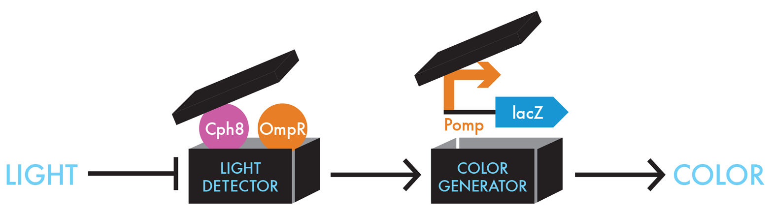
Figure 8-8. Unpacking the black box devices. To detect light in E. coli, the iGEM team genetically fused a portion of a light-sensing protein from cyanobacteria, Cph1, with the portion of the E. coli protein creating a novel protein, Cph8 (pink circle) that can phosphorylate OmpR (orange circle). The Cph8/OmpR combination can sense light as an input and then generates an output signal that can be understood by the Pomp-lacZ color-generating device.

EnvZ normally conveys information about salt concentrations outside the cell to OmpR by adding a phosphate to it. Phosphorylated OmpR can then bind the DNA just upstream of a particular promoter sequence and increase transcription of the gene downstream from that promoter. In nature, the genes regulated by phosphorylated OmpR encode membrane pores that allow more or less salt into the cell from the environment. In designing the bacterial-photography system, the iGEM team engineered the DNA so phosphorylated OmpR would regulate expression of β-gal. The team simply placed the OmpR-regulated promoter upstream of the lacZ gene, so OmpR would regulate lacZ as if it were a gene for a membrane pore (Figure 8-9).

About now you might be thinking, “Wait a minute... doesn’t this arrangement generate color in response to salt changes in the cell’s environment?” The goal was to sense light. There is no natural light-sensing protein in E. coli, so here, again, the iGEM team cleverly made use of some natural genetic elements. Cyanobacteria is a microbe that responds to light, and the iGEM team decided to modify a light-sensing protein from a cyanobacteria to report on light inputs in its E. coli system. The team made a genetic fusion that started with the gene for the light-sensing protein, Cph1, and ended with the portion of E. coli’s EnvZ that communicates with OmpR. Knowing that proteins divide the work they do into discrete modular domains, the iGEM team took a leap of faith that this fusion protein would work and that it would both sense light and communicate with OmpR as it hoped.

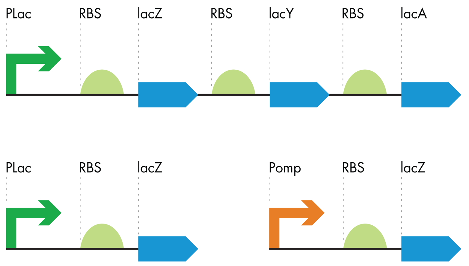
Figure 8-9. Making the color-generating device. The lac operon (top) was truncated (lower left) and modified with an OmpR-sensitive promoter (orange arrow) to generate a color-generating device that is sensitive to the OmpR protein.

To build its system, the team relied on genetics and molecular biology (as well as a ton of hard work and a measure of good luck) and it found a variant that could do all that the design needed it to do. The team called this fusion protein Cph8 (Figure 8-10). Like the Cph1 protein, Cph8 was sensitive to a particular wavelength of red light. To make it work, however, the team needed some “accessory” chromophores from cyanobacteria, so one more time the system was revised. In this newer version, the team expressed the cyanobacterial genes, ho1 and pcyA, which synthesize these accessory factors needed by Cph8.

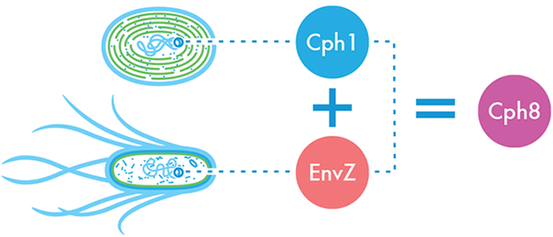
Figure 8-10. The light-sensing Cph8 fusion protein. A light-sensing protein from cyanobacteria, Cph1, was fused with the portion of the E. coli protein EnvZ that phosphorylates OmpR, creating a novel protein, Cph8, that takes light as an input and outputs a signal that can be understood by the Pomp-lacZ color-generating device.

When these final modifications were in place, the resulting system could express β-gal when the cells were grown in the dark. A red light source inhibited the phosphorylation of OmpR, leading to less transcription of LacZ and, consequently, less of the β-gal enzyme. Regions of a bacterial lawn could be shielded from light by growing the cells behind an image printed on a transparency and taped to the dish. The cells grown behind the dark part of the mask could turn the media around them black (Figure 8-11). Cells exposed to red light left the media its natural color, allowing the image on the mask to be reproduced in the media itself after a 24-hour growth period.

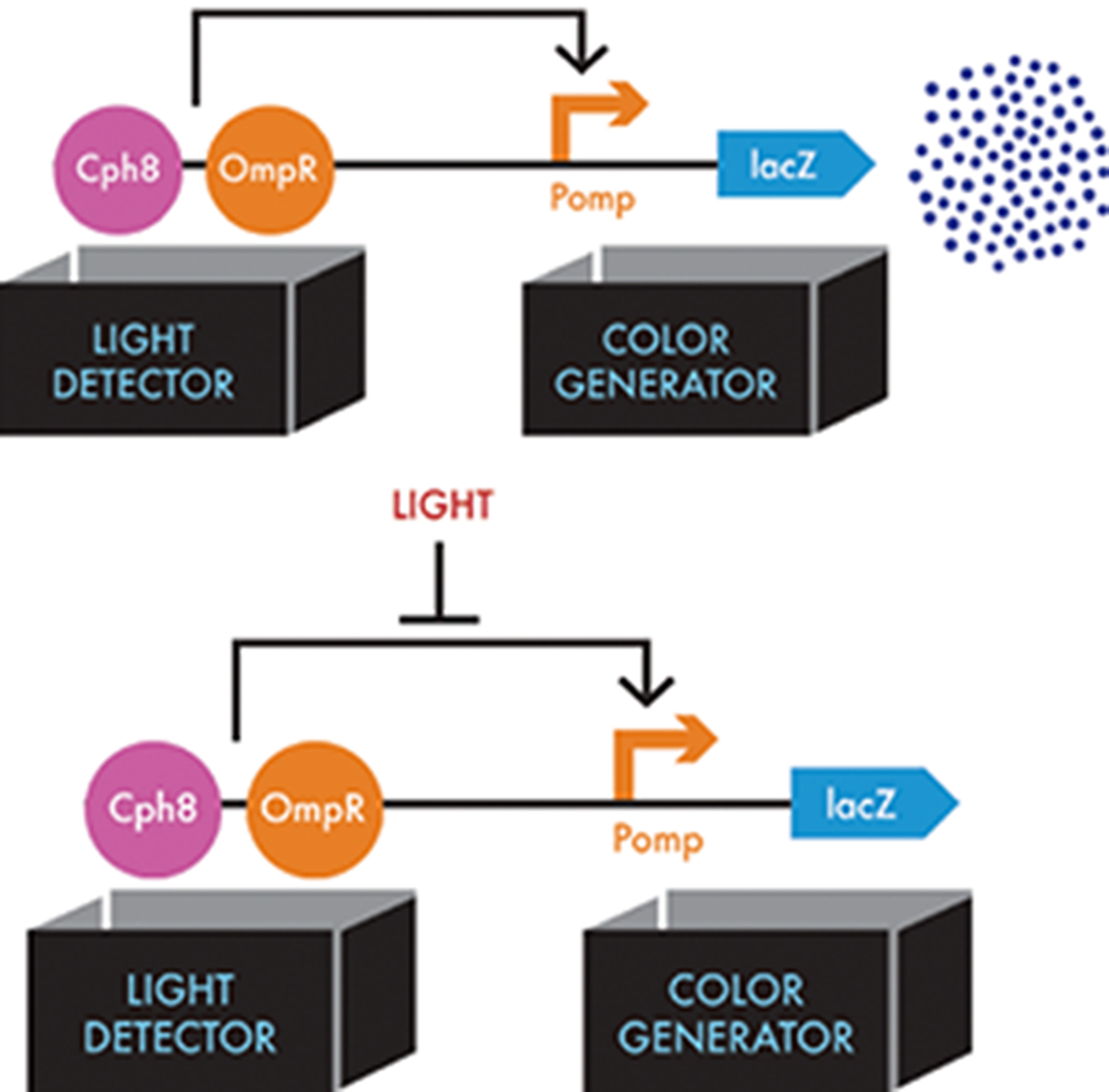
Figure 8-11. Information flow through the bacterial photography system. The light detector consists of the Cph8 fusion protein (pink circle) and the cell’s natural copy of OmpR (orange circle), which the Cph8 activates. In the top figure, activated OmpR can then bind to the Pomp operator (orange bent arrow) in the color-generator device, which results in lacZ expression (blue dart). In the bottom figure, when light shines on the system, this interaction of OmpR with Pomp is blocked (flat-headed arrow).

Additional Reading and Resources

§ Deepak, C., Bergmann, F.T., Suaro, H.M. TinkerCell: modular CAD tool for synthetic biology. J Biol Eng. 2009;3:19. Website: http://www.tinkercell.com/.

§ Levskaya, A. et al. Synthetic biology: engineering Escherichia coli to see light. Nature 2005;438(7067):441-2.

§ Stock, A.M., Robinson, V.L., Goudreau, P.N. Two-component signal transduction. Annual Review of Biochemistry 2000;69:183-215.

§ Website: BioBuilder “project” page on the Mouser Electronics site, where you can purchase each electronic part. (http://bit.ly/biobuilder_mouser).

Picture This Lab

BioBuilder’s Picture This lab introduces complex biological concepts, such as signaling transduction and cellular dynamics, through analysis of a modified two-component sensing system. It emphasizes the engineering concepts of abstraction and modeling with computer simulations of the engineered cell and through building an electronic circuit that is analogous to the cell’s genetic circuit.

Design Choices

Here, we use two approaches to understand the bacterial photography system: computational modeling with a program called TinkerCell and physical modeling with standard electrical components. In contrast with other BioBuilder activities, this lab focuses on developing experimental questions rather than asking them directly. The two complementary modeling approaches provide insight into different aspects of the living system’s behavior and illustrate the power and the shortcomings of our current efforts to model biology.

Although there is currently no “wet lab” component to the Picture This activity, supporting institutions can develop bacterial photographs made from the engineered strain by using an image of your choosing. Be sure to check the BioBuilder website for updates to this activity and to find submission guidelines. The protocol for developing bacterial photographs is described briefly in the following section.

Bacterial Photographs

To prepare bacterial photographs, the engineered strain is grown in the presence of the appropriate antibiotics that select for the light-detecting device, for the color-generating device, and for the auxiliary components that make the light sensor (Cph8) function in E. coli. You can then mix the overnight culture with molten agar, antibiotics, and the indicator compound, S-gal, and pour it into petri dishes to embed bacteria in the development media. You can tape a transparency with a black-and-white image to the back of the petri dish and then incubate it under red light overnight, giving time for the bacteria growing in the dark to produce the β-gal enzyme. Because the S-gal component of this media is quite expensive (~$600/gram) and because the wavelength of light that exposes these photographs is not standard, the most common way BioBuilder classrooms develop photographs is to send a transparency or a .jpg file of the image to be developed.

The most dramatic bacterial photographs result when cells grow in distinctly light or dark. If the black-and-white portions of the image are highly intermingled (an image with very fine lines, for instance), light can bounce around edges and blur the resulting photograph. In general, it’s better to have a dark background and a light image rather than the other way around. To darken the dark parts of the image, it’s common to print the same image on two transparencies and then overlay the two copies, using them both to mask the petri dish. The diameter of the petri dish is less than 3 inches across, so the image that’s selected must be smaller than this or adjusted to fit.

TinkerCell Modeling

You can download TinkerCell from the TinkerCell homepage. You can find detailed instructions for building the bacterial photography system in the TinkerCell platform as well as suggested simulations at the BioBuilder website.

The TinkerCell activity has two stages: redrawing of the bacterial photography circuit, and simulation of its behavior. As a first step in the redrawing stage, from the menu of parts that are available, you select the DNA circuit components for the devices and drop them onto the modeling canvas. In TinkerCell, these parts are categorized in terms of their functions; for example, “activator binding site,” “RBS,” “promoter,” “coding,” “transcription factor,” or “receptor.” Here is the list of components needed to model the bacterial photography system:

§ Components for the color-generator device:

§ Activator binding site

§ ompC promoter

§ ribosome binding site (RBS)

§ Coding region

§ β-galactosidase enzyme

§ Components for the light-detecting device:

§ Cph8 light receptor

§ OmpR transcription factor

§ Three “small molecules”:

§ S-gal

§ Color

§ Light

§ One cellular chassis

This model emphasizes the aspects of the system that we are most interested in, namely the transcriptional control of the β-gal enzyme. That is why some elements of the system, such as OmpR, are placed into the model as pre-existing proteins rather than as transcriptional gene-expression cassettes. Certainly there is transcriptional control and translational control of the elements we’ve put in as proteins, but the model here makes the assumption that these steps can be simplified and the control of them can be ignored for now. This simplification is another example of abstraction, an engineering tool discussed extensively in the Fundamentals of Biodesign chapter. We use abstraction here to keep the computational load manageable.

After choosing the components that go into the model, the next step is to explicitly define their relationships. Here is the list of relationships between the components to model for the bacterial photography system:

§ Cph8 can activate or inhibit its phosphorylation of OmpR (note that depending on which you choose, you will need to adjust whether light activates or inhibits Cph8).

§ Phosphorylated OmpR can bind to the activator binding site for the reporter gene.

§ The reporter gene can produce the β-gal enzyme.

§ β-gal can take the “S-gal” small molecule as input and can produce the “color” small molecule as output.

Finally, the chassis is added to the canvas. You must arrange the existing components so that the “light” small molecule is outside the cell, the Cph8 protein is in the cell membrane, and everything else is inside the cell (Figure 8-12).

The next stage in the TinkerCell activity is to run a simulation of the system’s behavior. Because the system is designed to be sensitive to light, the model’s output will stay the same unless the amount of light input changes. If the light is unchanged, remaining either on or off through the entire simulation, the model’s output will not change. You can specify when and how the light input changes using a step function in the TinkerCell menu options, and then you can run the simulation to see how the system responds to different light levels.

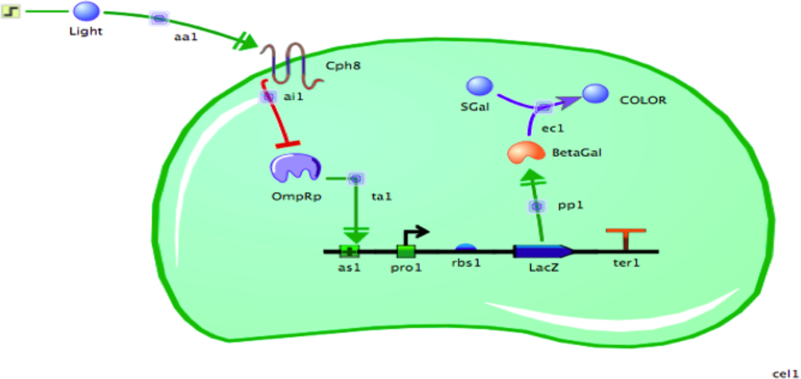
Figure 8-12. A screenshot of the TinkerCell modeling interface. This computational model of the bacterial photography system contains all of the genetic and biological components necessary to simulate the system’s behavior under various conditions.

TinkerCell provides default values called starting conditions that determine the starting concentration and reaction efficiencies for the model’s components. The enzymatic efficiencies are given a value, as are the strengths of the RBS, the promoter, the activation, the inhibition, and the amount of naturally occurring OmpR and S-gal available. When running the simulations, you can use the default values or you can change them to see how the model predicts the cell will respond. For example, what if there were 10 times more phosphorylated OmpR protein? If the amount of phosphorylated OmpR that binds the DNA had been limiting, the increase should result in more lacZ transcription and thus more β-gal enzyme. This change can, in turn, increase the amount of color formed in a limited amount of time if the enzyme’s catalysis of S-gal to make color is limiting.

So, even though TinkerCell makes many assumptions about the model’s components, you can adjust these parameters as a way to explore how the system might respond. You’ll find that these simulated experiments take a lot less time than the wet-lab version of them; therefore, if the model is set up well, it can save you many days at the bench and you take a smart experimental approach when you work there.

Electronic Circuit Modeling

In the physical modeling component of Picture This, you will build an electronic version of the bacterial photography strain. Recall from the architectural example from earlier in the chapter, a computer-aided design tool can help an architect evaluate and test a design under a wide range of environmental conditions. The architect might also undertake a complementary form of modeling, namely a physical model, to help envision the design and to identify needed but missing components. For synthetic biologists, a physical model of a cell might not provide much additional information, but a physical model that illustrates information flow through a genetic circuit can be informative and you can then use it to make test predictions about the circuit. As genetic circuits become more complex, modeling the flow of information through them can become impossibly difficult. The bacterial photography system, however, has a reasonably simple logic, and so we can use it to illustrate the value of a physical model, one that uses electronic components to “stand-in” for the biological ones, as demonstrated in Figure 8-13.

The section “Additional Reading and Resources” earlier in the chapter includes a link to the BioBuilder “project” page on the Mouser Electronics site, where you can find the electronic parts for this activity. Table 8-1 lists the components that are used specifically in this BioBuilder activity.

In the electronic system, a switch controls the current entering the circuit and so is analogous to the role played by the membrane-bound light-sensor protein (Cph8), which detects light and initiates or inhibits a kinase reaction. The behavior of the light-emitting diode (LED) mimics the output of the bacterial photography system by turning on or off depending on the state of the “light detecting” switch component of the circuit. The breadboard, wires, and resistor propagate the signal from the switch and specify the logic of the system, turning off the output when the switch is pressed on, and turning it on when the switch is off. The resistor also models the sensitivity of the system, regulating the amount of information flow through the system.

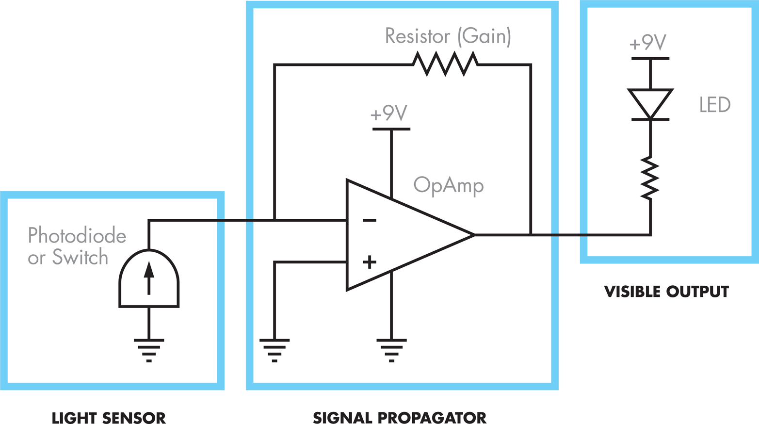
Figure 8-13. A schematic representation of the bacterial photography system electrical model. The light sensor (left), which is either a photodiode or a switch, corresponds to the light-detecting device. The visible output (right), an LED (light-emitting diode), corresponds to the color-generating device. A variety of components can connect the light detector and the LED to model signal propagation that occurs within the cell.

BUILDING CIRCUITS ON A BREADBOARD

A breadboard is a platform for rapidly prototyping electronic circuits. You can insert wires into the holes in the breadboard’s plastic cover to easily make electronic connections and test multiple circuit configurations.

But how do the holes connect the components together? The breadboard has two rails, one running along each side, which are the long columns marked with red or blue lines and plus or minus signs. It also has interior holes that are arranged in rows of five. The rails along the sides are where the circuit connects to power source and the ground of the power source. Grounding is essentially a way to return electrical current to the starting point, also known as closing or completing the circuit (for AC-powered systems outside of North America, you might see the term “earth” used in place of “ground”). If a circuit is not grounded, current cannot flow and the circuit will not function. The two rails on the breadboard are functionally identical, and so the circuit’s orientation is determined by connecting one rail to the power source and the other rail to ground.

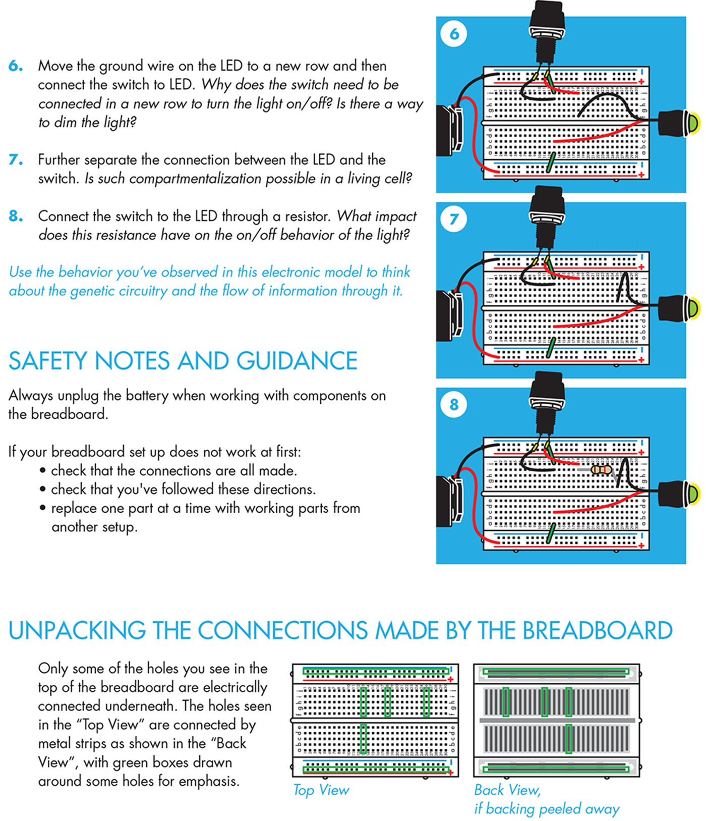
If you were to peel back the cover that’s behind the breadboard, you’d see the metal strips that sit behind the holes on the plastic breadboard (Figure 8-14). The metal connects the entire length of each rail, so you can connect the power and ground anywhere along the rails and the entire rail then provides either power or grounding. More metal strips also sit behind the five holes in each row, so they are connected to one another, but they are not connected to the holes in the next row or to the holes on the other side of the groove, or trench, running down the middle of the breadboard. Any electronic components inserted into holes in the same row are electrically connected, and current can flow between them (see http://bit.ly/building_circuits).

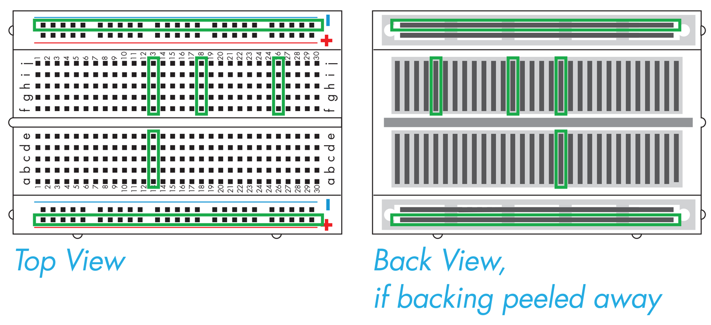
Figure 8-14. Electronic breadboards. A breadboard with the plastic top (left) and with its backing removed (right) to show the configuration of the conducting metal. The green outlines on the left correspond to the direction of the metal pieces, as shown on the right, and therefore reflect connectivity of the electronic components.

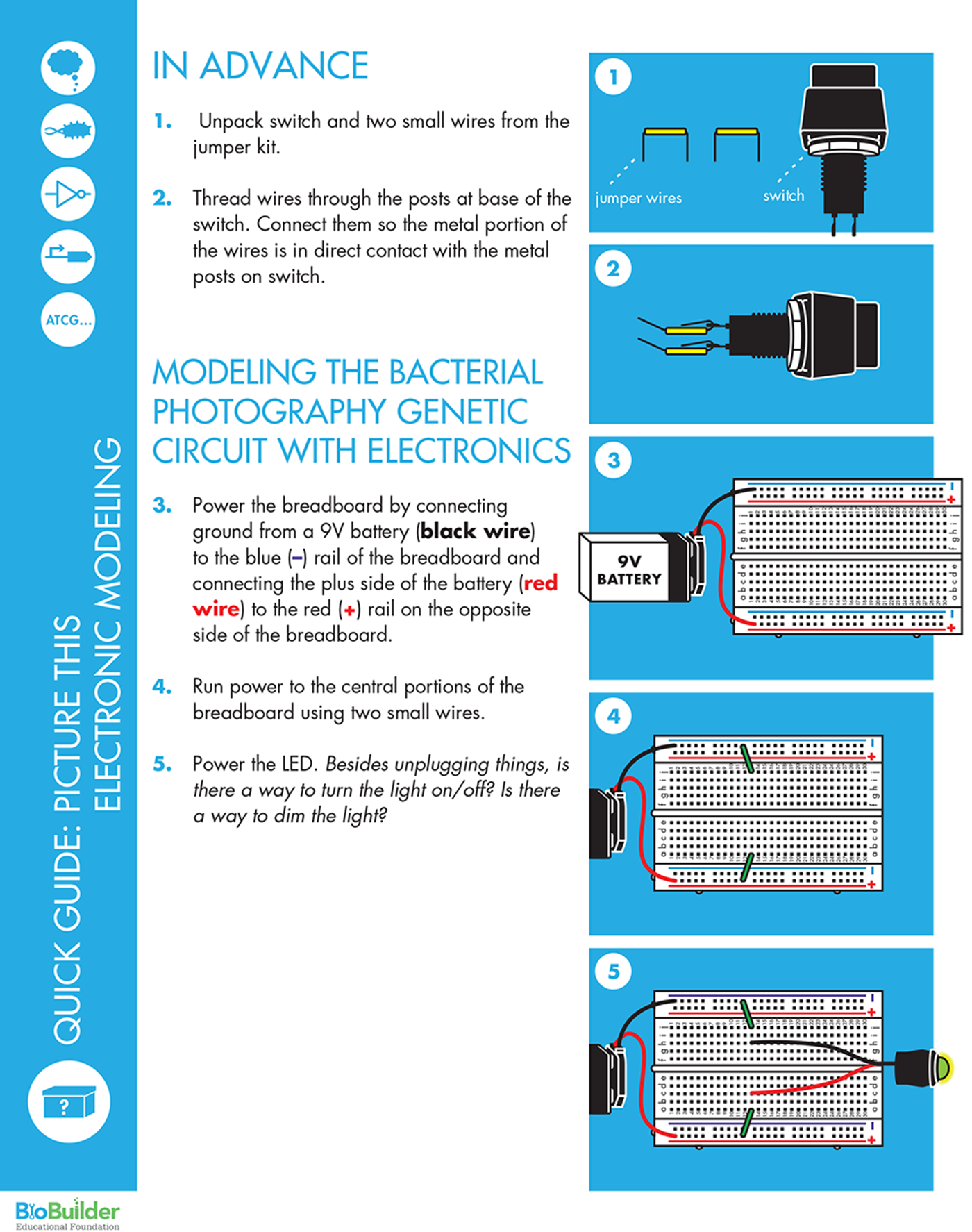
In electronics, red is traditionally used to indicate the positive pole and black the negative pole. Circuits require an energy source such as a battery, which can be connected to the breadboard via the binding posts. For this BioBuilder activity, the breadboard is powered by connecting the red wire from the 9V battery lead to one of the red (+) rails, and the black wire from the battery lead to the blue (-) rail on the other side of the board.

Electronics modeling activity

If you have the electronic components in hand to build the bacterial photography circuit, you can try the following.

First, power the breadboard by connecting ground from a 9V battery to the blue (-) rail of the breadboard and connecting the plus side of the battery to the red (+) rail on the opposite side of the breadboard. Next, run power to the central portions of the breadboard (where the rows with five holes are found) using two small wires. Finally, power the LED by connecting its red wire to the holes of the breadboard that are connected to the red rail and the LED’s other wire to the grounded side of the breadboard.

With this simple circuit, unplugging the leads is the only way to change the system’s output. To build a system that’s more easily changeable, you can add a switch to the circuit by moving the ground wire on the LED to a new row and then connecting the switch between the grounded row and the row with the LED ground wire. This is a good moment to note how easily the elements of the circuit can be rewired and how reliably they can be connected to communicate with one another. It’s also an opportune time to note that the switch we are using is digital (it’s either fully on or fully off), so the output can’t be “tuned.”

To modify the system’s output, the electronic circuit also includes a resistor. Though the circuit still exhibits switch-like behavior, you can change the intensity of the output by further separating the connection between the LED and the switch, and inserting a resistor between them. Use the behavior you observe to think about the genetic circuitry and points that can affect in the flow of information through each.

In teaching this activity in the past, we’ve noticed a few things that might help you if you’re trying this for the first time. When the electronics do not behave as expected, it useful to check that the connections have all been made according to the directions. Most times, a wire is misplaced on the breadboard. When the wiring is fully correct but the circuit still fails to function, it helps to swap parts one-by-one with a working setup. We have been frustrated by dead batteries, burned-out LEDs, and faulty breadboards, but you can identify and solve each problem by systematically exchanging parts between a failed and a working setup.